The impact of indoor solid fuel use on the stunting of Indian children

The impact of indoor solid fuel use on the stunting of

Indian children

ANCA BALIETTI

∗

Harvard University

SOUVIK DATTA

†

University of Glasgow

March 30, 2017

Abstract

About half of Indian children under the age of three years are stunted. We use data

from the 2005-2006 National Family Health Survey in India to assess the link between

being exposed to household air pollution from burning solid fuels and child stunting.

We tackle the endogeneity issue between child stunting and household fuel choice with

the help of an instrumental variables approach. Moreover, we study the potential het-

erogeneous impacts of household air pollution and other driving factors on stunting in

a quantile regression setting. We ﬁnd strong evidence that exposure to solid fuel smoke

increases the probability of being stunted and severely stunted among Indian children,

as well as reduces the height-for-age measure for those children. Our results also indi-

cate that the impact is stronger in the central part of the height-for-age distribution, and

not so much in the extremes. Given that this is where the vastest number of children are

situated, our results point also to the large scale of the required policy intervention. In-

centivizing a diminished exposure to household air pollution is expected to be no small

undertaking that targets only some pockets of the population, but rather a pan-Indian

project.

Keywords: Indoor air pollution; solid fuel; stunting; height-for-age score; instrumental

variables; ventilation.

JEL Classiﬁcation Codes: C35, C36, I15, I18, I32, I38.

∗

Center for International Development, Harvard Kennedy School of Government. <anca_balietti@hks.

harvard.edu>

†

Corresponding author: Adam Smith Business School, University of Glasgow, West Quadrangle, Gilbert Scott

Building, Glasgow G12 8QQ, Scotland. Phone: +44 141 330 6965. <[email protected]>

1 Introduction

The reliance on solid fuels for cooking and heating in developing countries has exacerbated

the problem of disease among their populations (Fullerton et al., 2008). The combustion of

solid fuels releases particulate matter consisting of carbon monoxide, benzene, formalde-

hyde, and other toxins into the surrounding air (Smith, 2000, p. 13287). The by-product of

these toxins are damaging to the health of individuals exposed, with problems compounded

by the lack of adequate ventilation in indoor areas. Studies have shown that exposure levels

in unventilated households using solid fuels are 10 – 50 times greater than exposure in ven-

tilated or outdoor areas (Smith, 2000, p. 13287). Moreover, household air pollution (HAP)

levels signiﬁcantly depend on the type of fuel used for cooking and heating, with some fu-

els generating up to ten times more particle matter than others (Smith et al., 2011). Solid

fuel types include wood products, agricultural crop residue, and animal dung; cleaner fuels

(non-solid) consist of electricity, liquid petroleum gas, and biogas.

Among the studies that analyze the negative health consequences of being exposed to

HAP caused by burning fuels, a plethora of them highlights the contribution to acute respi-

ratory problems (Pandey et al., 1989; Armstrong and Campbell, 1991; Mishra and Retherford,

1997; Sharma et al., 1998; Smith, 2000; Ezzati and Kammen, 2001; Brunekreef and Holgate,

2002; Balakrishnan et al., 2002; Duﬂo et al., 2008; Torres-Duque et al., 2008; Tielsch et al., 2009;

Yu, 2011; Prasad et al., 2012; Upadhyay et al., 2015).

This study focuses on India where HAP is a major health concern and ranks third in risk

factors for disease, behind high blood pressure and high blood sugar (Forouzanfar et al.,

2015). In India, children are particularly vulnerable to the harmful effects of indoor air pol-

lution due to their tendency to stay indoors and be carried by their mothers while cooking

(Mishra and Retherford, 2007, p. 377).

In this paper, we focus on a particular health impact of solid fuel use, namely its link

with child stunting. Stunted growth is at an alarmingly high level in India; based on the

1998 National Family Health Survey (NFHS-2), about half of the Indian children under three

years of age were displaying severely reduced height-for-age ratios (Mishra and Retherford,

2007). More worryingly, despite high economic growth during the last few decades, the

propensity for stunting seems to have remained at high levels in India, possibly signaling

that (i) India’s growth is not inclusive and does not beneﬁt the poorest part of the society

where stunting tends to prevail, or that (ii) there are some sticky drivers of stunting, such as

everyday family cooking and eating practices, that are well rooted in family or community

culture and do not change with income variations. In support of the weak link between

income growth and stunting rates, Vollmer et al. (2014) show that among the 36 countries in

their sample (including India), no signiﬁcant association can be found between the change

in per capita GDP and the change in the percentage of stunted children over the 1990-2011

horizon.

Only a few studies so far have speciﬁcally focused on the link between stunting and

exposure to indoor air pollution. Mishra and Retherford (2007) use a multinomial logistic

regression approach to estimate the impact of solid fuel use on the predominance of anemia

and stunting among Indian children. Employing data from the 1998-1999 National Family

Health Survey, they ﬁnd stunting to be signiﬁcantly more prevalent among children from

households using solid fuels. Relying on a similar methodological approach, Machisa et al.

(2013) analyze the association between solid fuel use and stunting in children from Swazi-

land. The authors ﬁnd no signiﬁcant evidence of a negative impact of solid smoke on height-

to-age ratios after adjusting for child characteristics such as sex, age, birth weight, and pre-

ceding birth interval.

Our contribution to the literature is threefold. First, we analyze the most recent data

available from the 2005-2006 India’s National Family Health Survey (hereafter NFHS-3) for

children aged 3 years old and younger, and compare our ﬁndings with the related literature

that used the 1998-1999 data. While our main variable of interest is the burning of solid fuels

inside the house, we account for other possible causes of stunting that include residential,

parental, and child-speciﬁc features, as well as wealth and nutritional intake. Second, we opt

for an instrumental variables estimation approach. As households are likely to take decisions

that affect both child health and domestic purchases (such as fuel type for cooking) simul-

taneously, endogeneity concerns arise. The instrumental variables approach is employed in

this setting to help us tackle endogeneity issues, reduce the bias of the estimated coefﬁcients,

and identify the causal impact of cooking with solid fuel on the stuntedness of children. We

expect our study to deliver higher precision estimates of the impact of solid fuel on stunting

than previous literature. The estimation is ﬁrst focused on the conditional mean of stunting

and, second, on the conditional quantiles of stunting. Finally, as opposed to most previous

literature, we analyse the height-for-age score in addition to the binary stunted and severely

stunted measures. This allows us to check how household characteristics relate linearly to

the continuous HAZ measure, and not only their effect on driving HAZ beyond the stunting

thresholds.

We ﬁnd strong evidence that exposure to smoke from burning solid fuel leads to a lower

height-for-age ratio and can explain the prevalence of stunting and severe stunting among

Indian children. Being exposed to solid fuel smoke increases the probability of being stunted

by about 6.5% on average for Indian children below three years old. This effect is half as im-

pactful as following an inappropriate nutrition, which is the usual top concern when trying

to ﬁght stunting. Other contributing factors to reduced height-for-age are poor kitchen in-

frastructure, a higher child birth order, and low levels of mother’s education and health

status. Moreover, we ﬁnd that residing in rural areas is associated with reduced stunting,

possibly due to lower outdoor air pollution levels than in urban centers, as well as other

unobserved inﬂuences. The instrumental variables quantile regression results also indicate

that the impact of solid fuel is stronger in the central part of the height-for-age distribution,

while less so in the extremes. Given that this is where the vastest number of children are

situated, our results point also to the large scale of the required policy intervention. Pro-

viding incentives to attain a lower exposure to household air pollution is expected to be no

small undertaking that targets only some pockets of the population, but rather a pan-Indian

project.

The remaining of this paper is organized as follows. Section 2 introduces the outcome

variable and key statistics related to it in the Indian context. Sections 3 and 4 lay the foun-

dations for our theoretical and methodological approach. Section 5 provides details on the

dataset used and the key sample statistics. We present the main ﬁndings in section 6. Finally,

Section 7 concludes and, based on our ﬁndings, discusses some potential avenues to lower

households’ exposure to indoor air pollution and avoid severely reduced growth rates.

2 Measuring stunted growth

In a well-nourished and healthy population, there is a statistically predictable distribution of

height for children of a given age. The standard index used for physical growth – height-for-

age – reﬂects the long-term effects of malnutrition, and indicates the skeletal growth of the

child. The height-for-age (HAZ) measure is expressed in standard deviation units (Z-score)

from the median of a reference population, and is deﬁned in Eq. (1):

HAZ

Height

− Median(reference population)

Standard Deviation(reference population)

. (1)

where HAZ

is the height-for-age indicator of child i, whose height is given by Height

According to WHO standards, a height-for-age Z-score less than -2 indicates beging stunted,

while a negative Z-score of less than -3 indicates being severely stunted. We rely on the

most recent international reference population, which was released by WHO in 2006 (WHO

Multicentre Growth Reference Study Group, 2006).

The Z-score of the reference population

is normally distributed; then, a child in the reference population will have a chance of less

than 2.3% to be stunted (Imai et al., 2014).

In our analysis, we consider three alternative deﬁnitions of stunting. We rely on two

indicator variables (stunted and severely stunted) and the continuous height-for-age Z-score

(HAZ). First, using three different measures helps with examining the robustness of our

analysis regarding the measurement of stunting. Second, we intend to capture not only

the factors that contribute to pushing height-for-age behind a certain threshold, but also to

understand the sensitivity of the continuous height-for-age variable to different factors.

The new standard is based on children of non-smoking mothers, around the world (Brazil, Ghana, India,

Norway, Oman, and the United states) who are raised in healthy environments and are fed with recommended

feeding practices (exclusive breastfeeding for the ﬁrst 6 months and appropriate complementary feeding from 6

to 23 months).

Stunted children tend to have both physical and cognitive developmental delays, includ-

ing delayed walking, delayed speech development, and reduced school performance. They

also experience higher rates of mortality and morbidity, including diabetes and hyperten-

sion. Moreover, lower height-for-age levels tend to have suboptimal long-term consequences

for an individual’s welfare (Glewwe et al., 2001; Akresh et al., 2011). Hoddinott et al. (2013)

ﬁnd the number of years of education, the scores in aptitude tests, the characteristics of mar-

riage partners, and women’s age at ﬁrst birth to be on average lower for individuals that had

low height-for-age scores as children.

In India, a very high incidence of low height-for-age ratios has been documented, with

46% of children under three years of age being stunted according to the 1998-99 National

Family Health Survey (NFHS-2) (Mishra and Retherford, 2007). Our analysis relies on In-

dia’s National Family Health Survey (NFHS-3) conducted in 2005-2006.

Figure 1 shows the

distribution of the HAZ score in our sample. The incidence of stunting appears to be similar

to the 1999 levels, with about half of the Indian children younger than three years old being

classiﬁed as stunted. Moreover, an alarmingly high percentage (25%) is classiﬁed as severely

stunted. It is also concerning that the mean value of the HAZ score is very low and drawing

close to the stunting threshold.

0.0

0.1

0.2

−6 −5 −4 −3 −2 −1 0 1 2 3 4 5

HAZ score

Density

MeanHAZ Severe_stunting_threshold Stunting_threshold

Figure 1: Distribution of HAZ score for children 36 months old and younger in India, based

on NHFS-3. The vertical lines mark the sample mean, and the cut-offs for stunting at -2 and

severe stunting at -3.

The NFHS-3 is a nationally representative sample covering all 29 Indian states with an overall response rate

of 92.4%. The survey contains information on infant and child mortality, maternal and child health, nutrition,

anemia, and the utilization and quality of health and family planning services. NFHS-3 adopted a two-stage

sample design in most rural areas while a three-stage sample design was adopted in most urban areas. More

details about the survey and its design are provided in IIPS (2007).

3 A theoretical model of child health

Child nutrition status is determined by a complex set of factors (Fenske et al., 2013), some

intrinsic to the child (such as age and gender) and some characteristic to the family and

community in which the child is raised (such as maternal education and access to safe drink-

ing water). Following previous literature (Becker, 1981; Strauss and Thomas, 1998; Bassol

et al., 2007), we rely on a simple and widely diffused model to capture the demand for child

health. In a framework of unitary household models,

each household maximizes its to-

tal utility function by taking decisions regarding children’s health (S),

leisure (L), and the

consumption of goods and services (G). The optimization problem can be written as:

max

S,L,G

U(S, L, G; X

, µ) (2)

such that: B = p

· S + p

· L + p

· G (3)

where U is a continuous utility function, increasing in the inputs (S, L, and G), and quasi-

concave. X

is a vector of parental characteristics, such as mother’s years of education

and current employment status. µ denotes the unobserved heterogeneous preferences of

the household. Utility is maximized subject to a budget constraint captured in Eq. 3, where

B is the total household budget allocated to children’s health, leisure, and the purchase of

goods and services. p

is the price per unit of child health, such as the price of food for feed-

ing the child or the price of medicines in case the child gets sick. The unit prices for leisure

and goods and services are p

and p

, respectively.

Child health (S) is modeled as a production function that depends on household (X

child (X

), and parental (X

) characteristics:

S = f (X

, X

) (4)

Solving the optimization problem of the household (Eq. 2) will lead to an optimal child health

level (S

∗

) given by:

∗

= S

∗

, X

, B, p

, p

, µ) (5)

Equation 5 gives insights into the variables that impact child health. For instance, a higher

level of education of the parents (reﬂected in X

) would lead to a better health (higher

height-for-age). Our variable of interest – relying on solid fuels as primary cooking fuel –

enters the set of household characteristics (X

) and we expect that using solid fuels will

lead to a worsening in child health, i.e. a reduction in the height-for-age score.

Unitary household models assume that both parents have identical preferences, resources are pooled, and

decisions are taken jointly (Imai et al., 2014).

It is assumed that children are not decisions makers. Instead, parents take decisions that maximize chil-

dren’s health and nutritional status, given certain constraints.

4 Empirical methodology

In this section, we discuss the econometric models used to estimate the effects of different

types of cooking fuel (solid vs. non-solid) on child stuntedness. In a ﬁrst step, we assume

that the impact of being exposed to indoor pollution from solid fuels is constant over the

entire height-for-age distribution and estimate the mean impact on stunting. In Section 4.2,

we study the impact of solid fuel on different segments of the children population via a

quantile regression approach.

In order to estimate Eq. 5, we follow Chay and Greenstone (2003) and assume that the

impacts of explanatory variables are linear and additional. The general linear model of child

stunting has the following basic speciﬁcation:

= β

+ β

SolidFuel

+ β

+ ε

, (6)

The outcome variable, S

, captures the long-term nutritional status of child i, as indicated by

three measures. First, we rely on the continuous height-for-age score, with HAZ ∈ [−6, 6] in

our sample. The remaining two measures are constructed as dummy variables and reﬂect

whether or not child i is stunted (S

= 1 if HAZ < −2 and S

= 0 otherwise) or severely

stunted (S

= 1 if HAZ < −3 and S

= 0 otherwise).

is a vector of independent variables that determine child stunting, and include household,

child, and parental characteristics, i.e. X

= {X

, X

} from Eq. 4 and detailed further

in Section 5. State ﬁxed effects are also accounted for in the model in order to capture any

differences across states that may arise due to, e.g., state-speciﬁc policies or other unobserved

state-level factors.

is the main coefﬁcient of interest and captures the true impact of indoor air pollution from

solid fuel use on the stunting measure of child i. SolidFuel

is a binary variable that takes a

unit value if child i resides in a household that uses solid fuel as the main cooking fuel, and

zero otherwise. The ordinary least square estimator of β

requires that E[SolidFuel

· ε

] = 0

for a consistent estimation. If, in Eq. 6, there are omitted factors that covary with the solid

fuel variable, then the estimated coefﬁcients via least squares will be biased.

The next section explains why endogeneity is a likely problem for our estimation and

how we suggest to tackle it via an instrumental variables approach.

4.1 Instrumental variables estimation

In our setting, endogeneity concerns arise from two directions. First, households are likely

to take decisions that affect both child health and domestic purchases (such as solid fuel

types) simultaneously. One can think about a family’s resources (such as time or ﬁnances)

as being allocated between caring for children and obtaining the fuel needed for cooking. If

children are unhealthy, their parents might choose to spend less time outside gathering fuel

(especially solid fuel), and more time inside caring for the children. Tending to sick children

could also reduce cooking time. Second, the endogeneity concerns are reinforced by the fact

that the fuel choice variable only captures the main fuel used in the household at the time of

the survey, and is likely to suffer from random measurement error. As households tend to

rely on multiple fuel options, both solid and non-solid, we lack information on what enters

the fuel mix and in which proportion beyond the primary component, and whether this is

predominantly clean or less so. Overall, the potential existence of both omitted variables

and measurement error motivate us to rely on the instrumental variables approach in order

to tackle the endogenity that is likely to bring bias on all model coefﬁcients, not only of the

endogenous variable (Wooldridge, 1995).

Besides the theoretical evidence for endogeneity, we assess its presence in our model

via a series of tests. First, we run a test of randomization (Stock and Watson, 2003, p. 526),

which reveals that the binary variable SolidF uel

is not random. Second, following Chay and

Greenstone (2003), we examine the correlation between fuel choice and predicted outcome

variables (stunted indicator, severely stunted indicator, and height-for-age score). We ﬁrst

predict the outcome variable on all exogenous variables in the structural equation (Eq. 6),

excluding fuel choice. We then regress the predicted outcome variable values on fuel choice

and ﬁnd a strongly signiﬁcant relation, signaling once again that OLS is likely to lead to

severely biased estimates and reinforcing the choice for the IV approach. The results of the

two endogeneity tests are detailed in the Appendix.

The challenge that arises in implementing the instrumental variables approach is to ﬁnd

a strong and valid instrument, which is (i) signiﬁcantly correlated with the endogenous re-

gressor, after controlling for the exogenous explanatory variables of the structural equation

(relevance criterion), and (ii) uncorrelated with the error term of the main equation (exclusion

criterion); see Kennedy (2003). In other words, the instrument should be correlated with solid

fuel use, our endogenous variable, to satisfy the relevance condition, but affect child stunt-

edness only through its impact on solid fuel use in order to satisfy the exclusion criterion.

To ﬁnd a strong and valid instrument, the drivers of household’s fuel choice need to be

identiﬁed ﬁrst. The instrument will then be selected among the factors that inﬂuence the

choice of fuel, but do not impact child stunting directly. Each fuel type has its own private

cost, given by the sum of its ﬁnancial cost (purchase price) and its opportunity cost (the

foregone resources, such as own time needed to collect fuel). The ﬁnancial cost is oftentimes

zero for households living in rural areas that rely on solid fuels, as they get to collect it from

the commons. However, the opportunity cost in terms of collection labor time might be

large; gathering ﬁrewood can require up to six hours daily, depending on distance to forest,

forest density or degradation state. For other solid fuels, the opportunity cost is related to

their alternative uses: dung is a valuable fertilizer, while crop residues can serve as animal

fodder. In urban areas, where relying on commercial fuels is more common and non-solid

fuels are predominant, opportunity costs tend to be low compared to purchase prices, unless

the latter are lowered through governmental subsidies (Heltberg et al., 2000).

Besides ﬁnancial and opportunity costs, other factors have been found to play a signiﬁ-

cant role in the decision for fuel types. Cultural preferences

or a strong (sometimes religion-

driven) loyalty to traditional cooking methods can lead households to opt for a fuel type

instead of another. On the other hand, using non-solid fuels can be perceived as a symbol of

welfare and some households rely on it also to signal their higher social status. Although not

a widely spread factor yet, being aware of the negative health consequences of using solid

fuels can make households choose cleaner cooking fuels instead of traditional ones. Finally,

the choice is further driven by ownership of a stove that runs on cleaner fuels, such as LPG

and kerosene. Even when households have a strong preference for using non-solid fuels, the

initial costs of purchasing an appropriate stove can be prohibitive, especially in situations of

restricted access to credit (Gupta and K

ohlin, 2006). It is easy to see then that the private cost

of different fuel types varies widely across households. Moreover, each household chooses

the type and amount of cooking fuel ’by maximizing its utility subject to a ”virtual” or ”shadow”

price of energy which is unobserved and unknown, except to the household itself, and which varies

between households depending on household and village characteristics’ (Heltberg et al., 2000).

*** Modify from here to introduce the chosen instrument(s)***

The latter can be understood in terms of geographical proximity to the resource, such as

closeness to the forest (wood), to an agricultural zone (dungcakes and crop residues), or

to the market (kerosene and LPG). Fuel availability is likely to inﬂuence childhood stunting

only indirectly through the impact on fuel choice, making it a potential candidate for a strong

and valid instrument. We propose to proxy fuel availability by the share of houses that uses

solid fuel as main cooking fuel in a primary sampling unit (PSU), and use it as instrument

for the endogenous variable. We deﬁne the fraction of houses that uses solid fuel in the PSU

(Z) as:

Nr. households in PSU j, where child i resides, that use solid fuel as main fuel

Nr. households in PSU j, where child i resides

(7)

is constant for all children living in PSU j, i.e. Z

= Z

, ∀i ∈ [1, N

], where N

is the total

number of children in PSU j.

The proposed instrument satisﬁes the relevance criterion, being strongly correlated with

fuel choice, as illustrated by the results of the ﬁrst stage estimation; see Section 6. While

it is not possible to formally test whether the instrument satisﬁes the exclusion criterion in

our just identiﬁed model (with only one instrument for the endogenous variable) (Kennedy,

2003), the condition is fulﬁlled on theoretical grounds. The prevalence of solid fuel among

neighboring households is likely to capture the ease of fuel accessibility in the area (proxim-

Some foods are considered to taste better when cooked with solid fuels than with non-solid fuels, such as

chapati in India, Aung et al. (2016).

ity to source), without having a direct impact on childhood stunting.

The IV approach consists in a two-stage estimation of the following model:

SolidFuel

= γ

+ γ

+ ν

(8)

= β

+ β

SolidF uel

+ β

+ ε

(9)

In the ﬁrst stage, solid fuel use is regressed on the instrumental variable (Z

) capturing

the fraction of households relying on solid fuel for cooking in PSU

, and the set of exoge-

nous regressors, X

, to produce the predicted endogenous variable

SolidF uel

. In the sec-

ond stage, the dependent variable is regressed on the predicted

SolidF uel

and the vector

of exogenous variables X

. The IV method aims to isolate a part of the variation in the en-

dogenous explanatory variable SolidF uel

that is not inﬂuenced by the omitted variables, in

order to generate consistent estimates. The IV estimation is expected to produce unbiased

estimates of the true impact of being exposed to indoor air pollution from burning solid fuels

on childhood stunting.

4.2 Quantile regression models

The ordinary least squares and IV models presented above assume a constant association

between the explanatory variables and the outcome variable over its entire distribution. The

two models will be useful for estimating the mean impact of living in a household that uses

primarily solid fuels for cooking on a child’s malnutrition status. However, it is likely that

children will react differently to the exposure to solid fuels smoke, depending on where

they are on the distribution of height-for-age. Such heterogeneous effects of the explanatory

variable on the outcome variable can be estimated via a quantile regression (QR) approach,

which was ﬁrst introduced by Koenker and Bassett Jr (1978).

As detailed in Bassol

e et al. (2007), the QR approach has a number of advantages com-

pared to the OLS model, as it is less sensitive to outliers, it leads to more robust estimators

when the normality assumption is not satisﬁed, and it performs better when heteroscedas-

ticity is present.

The QR approach has been increasingly applied to understand the impact of different

drivers on child stunting in the recent literature. Focusing on child malnutrition in Senegal,

Bassol

e et al. (2007) ﬁnds heterogeneous distributional impacts of access to public infrastruc-

Recent studies, e.g. Chafe et al. (2015), point to the signiﬁcant contribution of burning solid fuels inside

to outdoor PM2.5 levels. This could raise doubts that the chosen instrument satisﬁes the exclusion criterion,

as ambient air quality can also impact child health and stunting rates. However, it has been estimated that

burning solid fuels inside contributes up to 10% to global ambient pollution, while the contribution to local air

quality depends on various confounding factors (such as topography and weather) and no conclusions have

been reached so far on the magnitude of these impacts. With this background, we assume that there are no

systematic spillover effects of indoor pollution to the average outside pollution level in the primary sampling

unit and maintain our position that the chosen instrument satisﬁes the exclusion criterion.

ture (such as safe water and health facilities) on child’s stunted growth. Burchi (2010) relies

on a QR approach to study the impact on child stunting of the mother’s education level

and nutrition knowledge in Mozambique. The study shows that, while mothers’ nutrition

knowledge reduces stunting among children at the lower end of the height-for-age distri-

bution, her formal education is more important for increasing height-for-age in the higher

quantiles. Similar results related to parents’ education and its impact on child stunting are

reported by Borooah (2005) in India, using data collected from 15,000 households in 1994. Re-

lying on the NHFS-3 of 2005-2006 in India, Kandpal et al. (2009) show that maternal health

and education are better able to reduce stunting at the lower end of the distribution than on

the upper end. Another study employing the NHFS-3 dataset is Fenske et al. (2013), who

study the association between various socio-economic factors and childhood stunting in the

lower quantiles (15% and 35%) of the height-for-age distribution of 0-24 month old Indian

Children.

The overarching message of all QR studies of child stunting is that policy interventions

should account for the differential impacts that driving factors may have on child nutrition

at different points of the height-for-age distribution. As Aturupane et al. (2011) explain,

some interventions might have very limited impacts for reducing the prevalence of stunting

on average, but could be highly impactful for children at the lower end of the height-for-

age distribution. With this motivation, we will employ the QR approach in our analysis to

ﬁrst assess the potential differential impact of being exposed to solid fuel smoke on child

stunting, and second formulate policy recommendations that account for this heterogeneous

relation.

5 Data

This section describes the variables employed in the empirical analysis. Key summary statis-

tics at the child level are captured in Table 1. Additionally, we divide the sample according

to two criteria: (i) the outcome variable, i.e. child’s stunting status as measured by an HAZ

score below -2, and (ii) the endogenous variable, i.e. the main fuel type used in the house-

hold for cooking (solid vs. non-solid fuels). Accounting for the two criteria, Table 1 includes

subsample summary statistics in order to highlight important differences between the sub-

groups.

First, Table 1 captures entire sample and subsample statistics for three outcome measures

that proxy child health: two binary variables capturing whether the child is stunted and

severely stunted, and the continuous height-for-age measure (the HAZ score). In our sample,

38% of the children are stunted while 16% are severely stunted. The average HAZ score is 1.5

points below zero. When distinguishing between children exposed and not exposed to solid

fuel smoke, we observe a signiﬁcantly higher prevalence of stunting and severe stunting in

the former subsample compared to the latter. This observation brings ﬁrst-hand support

to the hypothesis that there is a link between the exposure to solid fuel smoke and adverse

health impacts. Our analysis will try to clarify whether this link is causal or the solid fuel use

indicator is a proxy for other factors (such as general wealth) that can inﬂuence child health.

Second, Table 1 illustrates statistics of other variables that could potentially inﬂuence

childhood stunting. The main focus of this study is on the link between stunting and house-

hold air pollution. HAP levels vary signiﬁcantly according to the type of fuel used for cook-

ing and heating, with some fuels generating up to ten times more particle matter than others

(Smith et al., 2011). The NFHS-3 includes information on households’ primary fuel type

used for cooking.

Sorted by their pollution potential from highest to lowest, we divide

the fuel types into two broad categories: (i) solid fuel, including animal dung, agricultural

crop waste, straw/shrubs/grass, wood, charcoal, and coal/lignite, and (ii) non-solid fuel,

including kerosene, biogas, LPG/natural gas, and electricity.

Our dataset does not provide

information about the intensity of child exposure to solid fuels (as measured in hours of daily

exposure, for example ). Thus, we proxy exposure by an indicator of fuel type: solid versus

non-solid. In support of this, Ramaswamy et al. (2004) ﬁnd that the solid fuel indicator is a

good predictor of high concentrations of particulate matter in the living space.

Figure 2 illustrates the distribution of the HAZ score by solid fuel use in our sample.

While this graph does not imply any causation, it is quite striking to see the association of

solid fuel use with the HAZ score, as marked by the different average HAZ scores in the two

subsamples.

Figure 2: Distribution of HAZ score by main fuel type used in the household.

Considering the exposure to HAP as a potential factor for stunting, one also needs to

account for the cooking practices of the household which, directly or indirectly, may reduce

the exposure and impact of IAP. In particular, we account for possible measures of indoor

The survey asked each respondent “What type of fuel does your household mainly use for cooking?”.

The residual category of other fuels was excluded from the analysis.

ventilation and the conﬁguration of the cooking space. For this, we use binary variables

that denote whether the house has any windows and if the kitchen is separated from the

remaining living space. Finally, to control for other possible sources of indoor air pollution,

we include an indicator variable to signal whether the child is exposed to tobacco smoke in

the household.

Beyond the impact of household air pollution, our analysis attempts to account for other

variables that could potentially impact stunting. Based on previous contributions to the

literature, we group the controls into (A) residential, (B) childhood, and (C) parental charac-

teristics. As Table 1 indicates, the difference in means between the subgroups is signiﬁcantly

different from zero, for all considered variables, with very few exceptions. This indicates that

indeed the characteristics of the stunted are different than those of non-stunted children; the

same holds true regarding the differences between the group of children exposed to solid

fuels smoke and those not exposed to it.

A. Residential characteristics

Previous literature ﬁnds that stunting tends to be signiﬁcantly associated with various

household characteristics, such as family income, household crowding, house construc-

tion type, access to safe water, geographical region, and setting (urban or rural) (Shah

et al., 2003; Machisa et al., 2013; Fenske et al., 2011). As NFHS-3 lacks information on

actual family income, we proxy it by including several indicator variables capturing the

presence of durable assets (such as refrigerator, radio, water pump, etc.).

Table 1 shows that, in our sample, stunted children tend to live in households where (i)

solid fuels are the primary fuel type used, (ii) the cooking space is not separate from the

remaining living space in the house, (iii) the house is less likely to have any windows, (iv)

the house is located in a rural area, (v) the ﬂoor of the house is more likely to be made of

clay, soil, sand, or dung, (vi) household members are more likely to practice open defeca-

tion, and (vii) the family owns in general less durable goods.

B. Child’s characteristics

Previous studies ﬁnd age, gender, birth order, birth weight, and recent sicknesses to be

signiﬁcantly correlated with stunting (Jayachandran and Pande, 2015; Machisa et al., 2013;

Fenske et al., 2011; Mishra and Retherford, 2007; Adair and Guilkey, 1997). We control for

these characteristics and, additionally, include information related to the children’s recent

health history: whether they had fever and/or diarrhea in the two weeks prior to the sur-

vey.

The duration a child is breastfed is another factor found to have inﬂuence on the height-

for-age score. However, the sign of the relation is the subject of academic debate; see

the discussion in Section 6.The WHO recommends exclusive breastfeeding for the ﬁrst six

months of life. After that, children should receive nutritionally adequate and safe comple-

mentary foods, while breastfeeding should continue for up to two years of age or beyond.

We include an indicator that marks whether or not the child has been breastfed for a pe-

riod of time in line with the WHO recommendations.

Table 1 illustrates that our sample is gender-balanced, and includes children with ages 35

months and younger. In our sample, stunting appears to be more prevalent among older

infants and with a daily nutrition based on less varied food. WHO, in its guiding princi-

ples for complementary feeding of children, recommends that a breastfed child aged 6-23

months should be fed from 4 or more different food groups. We indicate the diversity of a

child’s diet by a binary variable, such that a value of 1 is assigned if a child consumed 4 or

more food groups in the last 24 hours, otherwise the indicator is zero.

C. Parents’ characteristics

An important role for the occurrence of stunting appears to be played by some characteris-

tics of the parents (Shah et al., 2003; Rayhan and Khan, 2006; Semba et al., 2008). Our anal-

ysis accounts for several aspects related to the mother, such as: body mass index, height,

an indicator signaling whether she is currently employed, and the number of years of ed-

ucation.

In our sample, it is striking that mothers have on average only primary education and less

than a third are employed at the time of the survey. Distinguishing between stunted and

non-stunted children, Table 1 identiﬁes the potential inﬂuence on stunting of the number

of years of mother’s education, whether or not she supplemented her diet with iron during

pregnancy, and her current smoker status.

Summing up, analyzing the key statistics in our sample, many socio-economic differences

arise between the children exposed to solid fuel and those not exposed to it. Our analysis

will control for these discrepancies and attempt to quantify the net impact of being exposed

to solid fuel smoke on child stunting.

The recommendation does vary for the developed world. In the US, the American Academy of Pediatrics

(AAP) recommends that a child be exclusively breastfed for the ﬁrst 6 months and should get complementary

food thereafter while supporting breastfeeding for the ﬁrst year.

In line with WHO recommendations, the food group categories considered are: (i) milk, cheese, yogurt or

other milk products; (ii) bread, noodles or other food made from grains; (iii) oil, fats, butter, or products made

from them; (iv) mangoes, papaya, or other Vitamin A rich fruits; (v) beans, legumes/lentils and nuts; (vi) other

fruits and vegetables (including green leafy vegetables); and (vii) eggs, meat, poultry, ﬁsh, and shellﬁsh (and

organ meats).

Table 1: Summary statistics of outcome and explanatory variables

Entire sample Stunting status Fuel type

Stunted Non-stunted Solid Non-solid

(N = 14,659) (N = 4,963) (N = 9,696) (N = 9,161) (N = 5,498)

Mean SD Mean SD Mean SD Mean SD Mean SD

I. Outcome variables

Stunted indicator (1

HAZ<−2

)

1,2

0.38 0.48 1 0 0 0 0.42 0.49 0.25 0.43

Severely stunted indicator (1

HAZ<−3

)

1,2

0.16 0.37 0.43 0.49 0.00 0.00 0.19 0.39 0.09 0.20

Height-for-age score (HAZ)

1,2

-1.50 1.62 -3.08 0.87 -0.54 1.16 -1.65 1.62 -1.04 1.53

II. Explanatory variables

A. Household characteristics (X

)

Household is using primarily solid fuel

1,2

0.74 0.44 0.83 0.38 0.69 0.46 1 0 0 0

Fraction of solid fuel use in PSU

1,2

0.77 0.34 0.83 0.30 0.73 0.36 0.93 0.15 0.30 0.31

Kitchen is separate

1,2

0.52 0.50 0.43 0.49 0.57 0.49 0.44 0.50 0.75 0.43

House has any windows

1,2

0.61 0.49 0.52 0.50 0.67 0.47 0.51 0.50 0.91 0.29

Rural residence

1,2

0.71 0.45 0.77 0.42 0.68 0.47 0.88 0.33 0.23 0.42

Nr. household members

6.82 3.25 6.80 3.21 6.83 3.27 7.05 3.28 6.16 3.06

Floor not covered

1,2

0.53 0.50 0.63 0.48 0.47 0.50 0.70 0.46 0.05 0.22

Open defecation

1,2

0.59 0.49 0.69 0.46 0.53 0.50 0.77 0.42 0.10 0.29

Indicator that house has bank account

1,2

0.11 0.31 0.08 0.27 0.13 0.33 0.06 0.24 0.24 0.43

Electricity

1,2

0.63 0.48 0.54 0.50 0.68 0.47 0.50 0.50 0.98 0.14

Radio

1,2

0.31 0.46 0.26 0.40 0.34 0.47 0.27 0.44 0.43 0.49

1,2

0.43 0.50 0.34 0.47 0.49 0.50 0.28 0.40 0.85 0.36

Telephone

1,2

0.12 0.33 0.07 0.26 0.16 0.36 0.05 0.23 0.33 0.47

Computer

1,2

0.02 0.13 0.01 0.08 0.03 0.16 0.00 0.04 0.07 0.25

Fridge

1,2

0.14 0.35 0.08 0.27 0.18 0.39 0.04 0.21 0.43 0.49

Bicycle

1,2

0.54 0.50 0.52 0.50 0.55 0.50 0.55 0.50 0.49 0.50

Motorcycle

1,2

0.20 0.40 0.13 0.33 0.24 0.43 0.11 0.31 0.46 0.50

Car

1,2

0.03 0.16 0.01 0.11 0.04 0.19 0.01 0.09 0.08 0.27

Thresher

1,2

0.02 0.15 0.02 0.12 0.03 0.17 0.03 0.17 0.01 0.11

Tractor

1,2

0.03 0.16 0.01 0.12 0.03 0.18 0.03 0.17 0.02 0.13

Mattress

1,2

0.61 0.49 0.54 0.50 0.65 0.48 0.52 0.50 0.87 0.34

Bed

0.87 0.34 0.86 0.35 0.87 0.33 0.85 0.35 0.91 0.28

Chair

1,2

0.52 0.50 0.42 0.49 0.58 0.49 0.40 0.49 0.86 0.35

Table

1,2

0.41 0.49 0.31 0.46 0.47 0.50 0.29 0.45 0.76 0.43

Pressure cooker

1,2

0.38 0.49 0.29 0.45 0.44 0.50 0.21 0.41 0.88 0.33

Electric fan

1,2

0.50 0.50 0.40 0.49 0.56 0.50 0.35 0.48 0.93 0.26

Sewing machine

1,2

0.20 0.40 0.14 0.35 0.23 0.42 0.13 0.34 0.39 0.49

Water pump

1,2

0.12 0.32 0.09 0.28 0.13 0.34 0.10 0.30 0.15 0.36

B. Child’s characteristics (X

)

Child’s age (months)

1,2

16.99 9.66 19.76 8.32 15.33 10.03 16.69 9.69 17.87 9.52

Male child

0.54 0.50 0.53 0.50 0.54 0.50 0.53 0.50 0.56 0.50

Birth order

1,2

2.80 1.90 3.07 2.02 2.63 1.81 3.08 2.04 1.99 1.12

Varied food

1,2

0.37 0.48 0.22 0.41 0.46 0.50 0.35 0.48 0.40 0.49

Breastfeeding according to WHO

0.84 0.37 0.84 0.37 0.84 0.37 0.89 0.32 0.70 0.46

Child had fever in the past two weeks

1,2

0.18 0.38 0.19 0.39 0.17 0.38 0.19 0.39 0.15 0.36

Child had diarrhea in the past two weeks 0.14 0.35 0.15 0.35 0.14 0.34 0.14 0.35 0.13 0.33

C. Parents’ characteristics (X

)

Mother’s BMI

1,2

19.87 3.24 19.29 2.86 20.21 3.41 19.25 2.63 21.64 4.08

Mother’s height

1,2

151.75 5.73 150.49 5.56 152.51 5.69 151.31 5.65 153.02 5.76

Nr. years of mother’s education

1,2

4.68 5.06 3.36 4.37 5.47 5.28 3.08 4.12 9.26 4.71

Mother is currently working

1,2

0.28 0.45 0.33 0.47 0.25 0.43 0.32 0.47 0.15 0.35

Mother took Iron during pregnancy

1,2

0.66 0.47 0.61 0.49 0.70 0.46 0.60 0.49 0.84 0.37

Mother is smoking

1,2

0.10 0.30 0.12 0.33 0.09 0.28 0.12 0.33 0.04 0.19

Notes: Reported statistics are representative for the sample used in the regressions models. The initial sample

size of NFHS-3 is of 51,555 children; however, due to missing observations of many control variables, the ﬁnal

sample size used in the empirical analysis is heavily restricted. The total sample size of 14,659 observations

contains complete information on all variables used in the analysis. Coefﬁcients reﬂect survey household

weights. The superscripts (1, 2) placed next to each variable mark whether the difference in means between

subcategories is statistically signiﬁcantly different from zero, such that a subscript of 1 indicates that, for that

speciﬁc variable, the difference between the mean of the stunted group and the mean of the not-stunted group

is signiﬁcantly different from zero; a subscript of 2 indicates that the difference between the mean of the group

exposed to solid fuel smoke and the mean of the group not exposed to solid fuel smoke is signiﬁcantly different

from zero.

6 Results

6.1 Mean impact of solid fuel smoke exposure on stunting

This section presents the empirical results from the estimation of the long-term nutrition

status of children, as measured by three outcome variables: an indicator of stunting, an

indicator of severe stunting, and the continuous HAZ score. For each of the three dependent

variables, we present the results from the linear estimation and the instrumental variable

approach. Table 2 presents the results of the six models. Below we provide an overview of

the factors that contribute to stunted growth, with an emphasis on the relationship between

stunting and the exposure to smoke from burning solid fuels. The robustness of the linear

probability models is strengthened by the results from logistic regression models of stunting

and severe stunting; see Table A.3 in the Appendix.

The results of the ﬁrst-stage instrumental variables regression are presented in Table 3.

As expected, the fraction of households using solid fuel in the same PSU has a strong and

highly signiﬁcant effect on the solid fuel use by a household in the same PSU. The value

of the F -statistic is far above the rule-of-thumb value of 10 used as standard for models

with one instrument for one endogenous variable. The test points to a strong instrument,

indicating that the IV results are not affected by weak-instrument bias.

Solid fuel as primary fuel type used in the household

Our main focus is on the link between a child’s nutrition status and the main fuel type used

in the household where the child resides. As the instrumental variable models reveal, we

ﬁnd evidence that being exposed to solid fuel smoke signiﬁcantly reduces the HAZ score

and increases the probability of being severely stunted.

Taking into account again the sample statistics in Table 1, we see that the difference in

means between the HAZ score of children exposed to solid and those not exposed to it is

0.61.

Moreover, the OLS model estimates that up to 0.13 score points (or 21.31%) of this

difference is due to exposure to solid fuel, after accounting for all other driving factors. Em-

ploying the estimate from the IV model, about 0.265 score points or almost 43.44% of the

difference between the HAZ scores is due to exposure to smoke from burning solid fuels.

Our results reinforce the ﬁndings of Mishra and Retherford (2007) that high indoor air

pollution levels can contribute to chronic nutritional deﬁciencies in young children. While

their conclusions were only based on correlations, the instrumental variables approach em-

ployed in our paper can ﬁnally ascertain the existence of a causal link. Moreover, as their

study was based on data collected 7-8 years prior to ours, comparing the two results also

highlights that, unfortunately, households’ reliance on solid fuel continues to negatively af-

The mean HAZ score is −1.65 for children exposed to solid fuel smoke, while the mean HAZ score is −1.04

for children not exposed to it.

fect children’s health and contributes largely to the prevalence of stunting. Over the last two

decades, the increase in international awareness regarding the negative impacts of house-

hold air pollution on health seems to not have been strong enough to motivate parents to

keep their children unexposed to indoor pollution.

The residential characteristics marking indoor ventilation possibilities are essential for

understanding the inﬂuence of solid fuel exposure on child stunting. We ﬁnd that the avail-

ability of windows in the house and having the kitchen in a separate room than the rest of the

living space signiﬁcantly reduce the prevalence of stunting and severe stunting, and increase

the HAZ score. It remains, however, difﬁcult to distinguish if these house conﬁgurations in-

dicate ventilation opportunities or if they merely constitute proxies of general household

health.

Other residential characteristics

Our results show that several residential characteristics play an important role for the preva-

lence of stunted growth. We reach three conclusions. First, residing in rural areas seems to

be associated with reduced stunting, after accounting for other socio-environmental factors,

possibly due to lower outside air pollution levels and lower population densities in villages

than in cities, and potentially other unobserved inﬂuences. With many studies focusing on

reducing indoor air pollution in rural households (Balakrishnan et al., 2004; Parikh et al.,

2001), our study points to the importance of addressing solid fuel burning in urban settings

as well, where the impacts are augmented due to higher outdoor air pollution levels.

Second, we control for other potential sources of health problems. For children living in

households that practice open defecation, the incidence of stunting is higher, but the associ-

ation is not statistically signiﬁcant. This ﬁnding is in contrast to recent studies (e.g. Spears

et al. (2013)) that underline the negative consequences of open defecation on stunting.

Third, there appears to be a reduced prevalence of stunting in wealthier households, as

indicated by the coefﬁcients of the durable goods (see Table A.2 in the Appendix).

Child’s characteristics

Controlling for childhood characteristics, our analysis reinforces previous ﬁndings that stunt-

ing is more prevalent among older children, who are higher in the birth order, who suffered

loose bowels episodes in the recent period, and are undergoing a poorly diversiﬁed diet.

Being higher in the birth order or having a twin can be associated with a tighter allocation

of available resources as families get bigger and a higher prevalence of stunting among later

born children. Moreover, cultural factors can again play a role, with Indian families tending

to show preference for ﬁrst borns (see Jayachandran and Pande (2015)).

Finally, we ﬁnd a negative relation between the duration of breastfeeding and child stunt-

ing. This health puzzle has been the subject of extended research that points to the existence

of reverse causality (Marquis et al., 1997; Simondon and Simondon, 1998) or omitted variable

bias (Atsbeha et al., 2015) when modeling the breastfeeding – stunting relation.

Parents’ characteristics

The parental features that signiﬁcantly reduce the prevalence of stunting are found to be re-

lated to parents’ health, as captured by the mother’s body mass index and her height, and

socially-environmentally driven, such as mother’s years of education. Moreover, children of

mothers who have taken iron supplements during pregnancy are less likely to be severely

stunted. The exposure to tobacco smoke does not appear to have statistical power in explain-

ing stunting for our sample.

Marquis et al. (1997) and Simondon and Simondon (1998) ﬁnd that mothers tend to prolong breastfeeding

for children that have poor growth and health. Atsbeha et al. (2015) control for the nutritional adequacy of

complementary foods and ﬁnd no evidence of adverse growth effects from prolonged breastfeeding.

Table 2: Regression models of stunting and severe stunting

LPM OLS IV

HAZ<−2

HAZ<−3

HAZ 1

HAZ<−2

HAZ<−3

HAZ

) (M

)

Intercept 2.277*** 1.236*** -8.694*** 2.266*** 1.215*** -8.623***

(0.147) (0.117) (0.475) (0.148) (0.117) (0.478)

A. Household characteristics (X

)

Household is using primarily solid fuel 0.045*** 0.017 -0.130** 0.065* 0.058** -0.265**

(0.017) (0.013) (0.054) (0.034) (0.026) (0.111)

Kitchen is separate -0.042*** -0.016* 0.088** -0.041*** -0.015* 0.087**

(0.012) (0.009) (0.037) (0.012) (0.009) (0.037)

House has any windows -0.034** -0.030*** 0.135*** -0.034** -0.030*** 0.134***

(0.013) (0.011) (0.042) (0.013) (0.011) (0.042)

Rural area -0.021 -0.018* 0.075 -0.026 -0.029** 0.110**

(0.014) (0.011) (0.047) (0.016) (0.013) (0.053)

Nr. household members 0.003* 0.000 -0.010* 0.003 -0.000 -0.009

(0.002) (0.001) (0.006) (0.002) (0.001) (0.006)

Floor not covered 0.005 0.005 0.020 0.003 0.002 0.031

(0.015) (0.012) (0.049) (0.016) (0.012) (0.049)

Open defecation 0.017 0.010 -0.027 0.014 0.004 -0.009

(0.016) (0.012) (0.049) (0.016) (0.012) (0.050)

B. Child’s characteristics (X

)

Child’s age 0.009*** 0.006*** -0.042*** 0.009*** 0.006*** -0.042***

(0.001) (0.000) (0.002) (0.001) (0.000) (0.002)

Male child -0.020** -0.013* 0.050 -0.019** -0.013* 0.049

(0.010) (0.008) (0.031) (0.010) (0.008) (0.031)

Birth order 0.002 0.006** -0.001 0.002 0.006** -0.002

(0.003) (0.003) (0.010) (0.003) (0.003) (0.010)

Diverse diet -0.137*** -0.062*** 0.466*** -0.137*** -0.063*** 0.467***

(0.011) (0.008) (0.036) (0.011) (0.008) (0.036)

Breastfeeding according to WHO 0.028* 0.039*** -0.197*** 0.028* 0.038*** -0.193***

(0.015) (0.012) (0.051) (0.015) (0.012) (0.051)

Had fever in the past two weeks 0.008 -0.004 -0.065 0.008 -0.005 -0.063

(0.013) (0.011) (0.041) (0.013) (0.011) (0.041)

Had diarrhea in the past two weeks 0.032** 0.013 -0.152*** 0.032** 0.013 -0.153***

(0.014) (0.011) (0.043) (0.014) (0.011) (0.043)

C. Parents’ characteristics (X

)

Mother’s BMI -0.009*** -0.004*** 0.039*** -0.009*** -0.004*** 0.038***

(0.002) (0.001) (0.005) (0.002) (0.001) (0.005)

Mother’s height -0.012*** -0.007*** 0.047*** -0.012*** -0.007*** 0.047***

(0.001) (0.001) (0.003) (0.001) (0.001) (0.003)

Nr. years of mother’s education -0.006*** -0.004*** 0.017*** -0.005*** -0.004*** 0.015***

(0.001) (0.001) (0.005) (0.001) (0.001) (0.005)

Mother is currently working 0.014 0.005 -0.040 0.014 0.004 -0.040

(0.012) (0.010) (0.039) (0.012) (0.010) (0.038)

Mother took iron during pregnancy -0.007 -0.031*** 0.050 -0.007 -0.031*** 0.050

(0.012) (0.010) (0.039) (0.012) (0.010) (0.039)

Mother is smoking 0.009 -0.008 -0.064 0.009 -0.008 -0.065

(0.018) (0.015) (0.056) (0.018) (0.015) (0.056)

Household assets Yes Yes Yes Yes Yes Yes

State ﬁxed effects Yes Yes Yes Yes Yes Yes

Nr. observations 14,659 14,659 14,659 14,659 14,659 14,659

0.157 0.106 0.207 0.157 0.105 0.207

Adj. R

0.153 0.101 0.203 0.153 0.101 0.203

Notes: The table capture estimation results from linear models of stunting (M

) and severe stunting (M

), OLS

model for the HAZ score (M

), and the IV models for each output measure (M

- M

). Errors were clustered

by household, and robust standard errors are presented in parentheses below each coefﬁcient. Signiﬁcance

levels are indicated by

∗∗∗

∗∗

∗

, marking the 1%, 5% and 10% levels, respectively.

Table 3: First stage regression of solid fuel use for the instrumental variables approach.

HAZ

)

Intercept 0.23***

(0.07)

Fraction of solid fuel in PSU 0.71***

(0.02)

A. Household characteristics (X

)

Kitchen is separate -0.01

(0.01)

House has any windows -0.00

(0.01)

Rural area 0.00

(0.01)

Nr. household members 0.01***

(0.00)

Floor not covered 0.05***

(0.01)

Open defecation 0.07***

(0.01)

B. Child’s characteristics (X

)

Child’s age 0.00

(0.00)

Male child -0.00

(0.00)

Birth order -0.01***

(0.00)

Varied food 0.01

(0.01)

Breastfeeding 0.02**

(0.01)

Had fever in the past two weeks 0.01

(0.01)

Had diarrhea in the past two weeks -0.01*

(0.01)

C. Parental characteristics (X

)

Mother’s BMI -0.00*

(0.00)

Mother’s height 0.00

(0.00)

Nr. years of mother’s education -0.01***

(0.00)

Mother is currently working 0.00

(0.01)

Mother took iron during pregnancy 0.00

(0.01)

Mother is smoking -0.00

(0.01)

Household assets Yes

State ﬁxed effects Yes

Nr. observations 14,659

First stage F -statistic 1,641.11

Prob > F 0.0000

Notes: Errors were clustered by household, and robust standard errors are presented in parentheses below each

coefﬁcient. Signiﬁcance levels are indicated by

∗∗∗

∗∗

∗

, marking the 1%, 5% and 10% levels, respectively.

6.2 Heterogeneity in impacts of solid fuel smoke exposure on stunting

This section explores the heterogeneity of child stunting determinants on the height-for-age

score. Analyzing the differential impact that household air pollution may have on stunting

at different points of the height distribution would allow us to draw conclusions regarding

which children should be targeted ﬁrst by policy interventions for stronger outcomes.

The unconditional distribution of the HAZ score is illustrated in Fig. 3; the vertical red

lines mark the values of HAZ at different quantiles of interest. The instrumental variable

quantile regression results are captured in Table 4; the coefﬁcients of some selected variables

of interest are illustrated graphically in Fig. 4. We ﬁnd that our variable of prime interest, i.e.

whether or not the household uses solid fuel as primary fuel for cooking, has signiﬁcantly

distinct impacts on the height-for-age variable at different quantiles of the distribution. Being

exposed to solid fuel smoke appears to signiﬁcantly reduce height-for-age mostly for the

middle of the distribution, i.e. for the 0.5, 0.75, and 0.90 quantiles, while the impact remains

not signiﬁcant at the distribution extremes.

Figure 3: Histogram of the sample HAZ score with markup at different distribution quan-

tiles.

On the left-hand-side of the HAZ distribution, for quantiles of 0.25 and lower, all children

are stunted or severely stunted, with an HAZ score below -2 (Fig. 4). It is likely that their

health is so weakened by other driving factors that being exposed to solid fuel has no signiﬁ-

cant additional impact. An alternative hypothesis is that such malnourished children are too

weak to spend long hours next to their mothers close to the cooking place and are, thus, less

exposed to solid fuel smoke. On the right-hand-side of the distribution, for the 0.95 and 0.975

The robustness of these results is conﬁrmed also the OLS quantile regressions models. Although coefﬁ-

cient signs and signiﬁcance tends to match between simple QR and IVRQ models, coefﬁcient magnitudes differ,

especially for the endogenous variable Solid Fuel. Results are captured in Table A.6 in the Appendix.

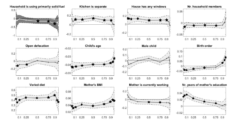
quantiles, where the HAZ score is 1.39 and higher, we again observe no signiﬁcant impact

of solid fuel smoke on the HAZ score. It appears that the height-for-age score is immune to

solid fuel smoke exposure among the healthiest children. Overall, the IVQR analysis reveals

that policy interventions regarding the switch from solid to cleaner fuels should be directed

neither at the weakest nor the healthiest Indian children. In contrast, most beneﬁts from

reducing the use of solid fuels would accrue to children in the middle of the height-for-age

distribution. Given that it is here where the vastest number of children are situated, our

results also point to the large scale of the required intervention. Incentivizing the switch to

cleaner fuels is expected to be no small undertaking that targets only some pockets of the

population, but rather a pan-Indian project.

Figure 4: Instrumental variable quantile regressions estimates of selected explanatory

variables for child’s height-for-age score.

Notes: The ﬁgure illustrates the estimated coefﬁcients for selected explanatory variables of the height-

for-age score. Results come from ﬁtting IVQR models for the {0.025, 0.05, 0.10, 0.25, 0.50, 0.75, 0.90, 0.95, 0.975}

quantiles. 90% conﬁdence intervals are depicted in gray. Statistically signiﬁcant coefﬁcient are marked with

black stars in the graph.

The IVQR analysis allows us to study the association of the height-for-age score with

other factors at different points of the HAZ distribution. The results for some selected vari-

ables of interest are illustrated in Fig. 4. We draw three conclusions. First, a determinant

that could potentially mitigate the impact of household air pollution on stunting is given by

ventilation options, such as cooking in a separate room than the rest of the living space and

having any windows in the house. Similarly to solid fuel, these two avenues for better venti-

lation have no signiﬁcant association with the HAZ score at the extremes of the distribution,

but do so for the more central quantiles.

Second, some of the variables that had no signiﬁcant impact on HAZ in the simple IV

models, turn out to play a signiﬁcant role for some parts of the distribution, among which

the number of household members, the open defecation indicator, child’s birth order, the

breastfeeding indicator, the number of years of mother’s education, and the indicator of

whether the mother is currently working. In particular, breastfeeding appears to have a ben-

eﬁcial impact on children at the bottom of the height-for-age distribution, but detrimental for

the higher quantiles; see again the discussion on the literature debate regarding breastfeed-

ing in Section 6.1. Although highly signiﬁcant in the simple IV regressions models, the IVQR

regression analysis reveals that the number of years of mother’s education is positively as-

sociated with child’s nutritional outcomes only for quantiles of 0.75 and below. In contrast,

it appears that, for the higher end of the HAZ distribution, maternal education plays no

signiﬁcant role.

Third, some representative variables that had a strongly signiﬁcant association with height-

for-age in the simple IV models continue to exhibit the same strong correlation over the entire

HAZ distribution, as highlighted by the IVQR models. In particular, child’s age, having a

diverse diet, and mother’s BMI and height covary positively with height-for-age at all con-

sidered quantiles.

Overall, the instrumental variables quantile regressions offer a more complete picture of

the relation between child’s height-for-age and the explanatory variables, and at times point

to the heterogeneity of this relation along the HAZ distribution. Any policy interventions

trying to correct the high prevalence of stunting among Indian children should take into

account the differential impacts of the driving factors. In particular, we have seen that the

switch towards cleaner fuels is expected to bring the highest beneﬁts if incentives programs

are directed towards the middle of the height-for-age distribution, where the sensitivity of

HAZ appears to be hights to the choice of the household fuel. Our results contrast to some

extent the ﬁndings of Fenske et al. (2013), who employ additive quantile regression mod-

els and study the link between socio-economic factors and childhood stunting at the lower

quantiles of the height-for-age distribution. The authors ﬁnd that the association of most

variables with stunting on lower quantiles is similar to their impact on the population mean.

We believe the difference is driven by the empirical approach choice, additive QR versus

IVQR; moreover, our study highlights that in order to reach a broader understanding of po-

tential heterogeneous associations between height-for-age and its driving factors, one needs

to consider the impact not only on lower, but also on higher quantiles.

Table 4: Instrumental variable quantile regressions of the HAZ score

HAZ Instrumental variable quantile regressions

Q = 0.025 Q = 0.05 Q = 0.10 Q = 0.25 Q = 0.50 Q = 0.75 Q = 0.90 Q = 0.95 Q = 0.975

) (M

)

Intercept -9.156*** -10.116*** -10.422*** -9.996*** -9.250*** -8.645*** -7.360*** -5.612*** -4.361***

(0.964) (0.774) (0.590) (0.429) (0.414) (0.466) (0.668) (1.035) (1.290)

A. Household characteristics (X

)

Household is using primarily solid fuel -0.135 -0.120 -0.025 -0.105 -0.165* -0.170* -0.320** -0.225 -0.435

(0.317) (0.181) (0.136) (0.096) (0.090) (0.095) (0.154) (0.255) (0.277)

Kitchen is separate 0.122 0.066 0.112** 0.110*** 0.143*** 0.095** 0.093* 0.010 -0.002

(0.093) (0.061) (0.049) (0.035) (0.032) (0.038) (0.055) (0.079) (0.115)

House has any windows 0.150* 0.130* 0.126** 0.131*** 0.092** 0.093** 0.103* 0.057 -0.035

(0.090) (0.077) (0.053) (0.040) (0.039) (0.043) (0.062) (0.088) (0.117)

Rural area 0.323** 0.261*** 0.096 0.092** 0.033 0.062 0.065 0.128 0.233*

(0.144) (0.087) (0.068) (0.046) (0.042) (0.049) (0.076) (0.113) (0.133)

Nr. household members -0.024 -0.017* -0.009 -0.011** -0.010** -0.012** -0.010 0.002 0.021

(0.015) (0.009) (0.007) (0.005) (0.005) (0.005) (0.008) (0.014) (0.017)

Floor not covered 0.064 0.008 0.035 0.023 0.011 0.028 0.134** 0.109 0.241

(0.097) (0.078) (0.063) (0.047) (0.042) (0.049) (0.067) (0.114) (0.162)

Open defecation -0.127 -0.135* -0.095 -0.091** 0.010 -0.033 -0.034 -0.056 -0.011

(0.108) (0.073) (0.063) (0.046) (0.045) (0.051) (0.075) (0.111) (0.164)

B. Child’s characteristics (X

)

Child’s age (months) -0.043*** -0.043*** -0.042*** -0.041*** -0.040*** -0.040*** -0.038*** -0.037*** -0.032***

(0.005) (0.004) (0.003) (0.002) (0.002) (0.002) (0.003) (0.004) (0.006)

Male child -0.008 -0.070 -0.056 -0.006 0.035 -0.028 0.033 0.060 -0.055

(0.068) (0.050) (0.040) (0.029) (0.027) (0.031) (0.047) (0.065) (0.098)

Birth order -0.027 -0.039** -0.044*** -0.030*** -0.018* -0.013 0.029* 0.059** 0.090**

(0.021) (0.018) (0.012) (0.011) (0.009) (0.011) (0.017) (0.027) (0.038)

Diverse diet 0.425*** 0.350*** 0.400*** 0.448*** 0.439*** 0.449*** 0.499*** 0.394*** 0.359***

(0.084) (0.057) (0.044) (0.031) (0.030) (0.035) (0.058) (0.084) (0.114)

Breastfeeding according to WHO 0.258*** 0.110 -0.041 -0.095** -0.065* -0.059 -0.237*** -0.374*** -0.514***

(0.100) (0.078) (0.058) (0.040) (0.038) (0.046) (0.077) (0.110) (0.149)

Had fever in the past two weeks -0.032 -0.048 -0.062 0.021 0.009 -0.064* -0.053 -0.106 -0.029

(0.093) (0.072) (0.056) (0.038) (0.036) (0.038) (0.064) (0.090) (0.151)

Had diarrhea in the past two weeks -0.140 -0.021 -0.004 -0.126*** -0.119*** -0.164*** -0.219*** -0.343*** -0.407***

(0.116) (0.076) (0.054) (0.042) (0.038) (0.045) (0.062) (0.083) (0.125)

C. Parents’ characteristics (X

)

Mother’s BMI 0.038*** 0.033*** 0.034*** 0.041*** 0.037*** 0.042*** 0.048*** 0.055*** 0.053***

(0.010) (0.007) (0.006) (0.004) (0.004) (0.005) (0.008) (0.012) (0.019)

Mother’s height 0.029*** 0.040*** 0.046*** 0.049*** 0.051*** 0.054*** 0.052*** 0.047*** 0.042***

(0.006) (0.005) (0.004) (0.003) (0.003) (0.003) (0.004) (0.006) (0.008)

Nr. years of mother’s education 0.030*** 0.032*** 0.036*** 0.023*** 0.013*** 0.008* 0.001 0.004 0.004

(0.011) (0.008) (0.006) (0.004) (0.004) (0.004) (0.007) (0.009) (0.013)

Mother is currently working 0.109 0.055 -0.004 -0.055 -0.065** -0.074** -0.080 -0.081 -0.106

(0.074) (0.060) (0.047) (0.035) (0.033) (0.038) (0.062) (0.082) (0.120)

Mother took iron during pregnancy 0.139* 0.099 0.105** 0.089** 0.048 -0.018 -0.087 -0.144 -0.204*

(0.078) (0.063) (0.049) (0.037) (0.034) (0.040) (0.059) (0.089) (0.115)

Mother is smoking 0.031 0.002 -0.046 -0.052 -0.039 -0.109** -0.126 -0.213* -0.102

(0.107) (0.089) (0.065) (0.050) (0.046) (0.050) (0.080) (0.112) (0.214)

Household assets Yes Yes Yes Yes Yes Yes Yes Yes Yes

State ﬁxed effects Yes Yes Yes Yes Yes Yes Yes Yes Yes

Nr. observations 14,659 14,659 14,659 14,659 14,659 14,659 14,659 14,659 14,659

Notes: The table captures estimation results from instrumental variables quantile regressions models of the height-for-age score. Errors were clustered

by household, and robust standard errors are presented in parentheses below each coefﬁcient. Signiﬁcance levels are indicated by

∗∗∗

∗∗

∗

, marking the 1%,

5%, and 10% levels, respectively.

7 Discussion and conclusions

The detrimental effects of indoor air pollution on children’s health are becoming increasingly

apparent, particularly on children living in India, where the prevalence of solid fuel use is

extensive.

We analyse the most recent data available from the 2005-2006 India’s National Family

Health Survey (NFHS-3) in order to determine what are the main drivers of stunting among

Indian children. In particular, we test whether the use of solid fuels for cooking and heating

is linked to the prevalence of stunting in children, and estimate the extent of the impact after

controlling for other confounding factors.

Stunting is not only a proxy for temporary health problems, but it indicates chronic mal-

nutrition and life-long wellbeing deﬁciencies. It has been shown to be associated with lower

educational outcomes and diminished life accomplishments. We believe it is, thus, highly

important to understand its drivers and implement policies to largely eliminate it.

Our analysis brings strong evidence that the exposure to solid fuel smoke leads to a lower

height-for-age ratio and can explain the prevalence of stunting and severe stunting among

Indian children. Other contributing factors are an urban setting, and the practice of openair

defecation. Stunting rates appear to be larger for children of older age, of higher birth order,

and who have been sick recently. Parental characteristics appear highly relevant for the

prevalence of stunting, such as mother’s height and body mass index. Moreover, stunted

children are associated to mothers with lower levels of education.

Our results reveal that households where indoor air pollution is likely to have lower con-

centrations, due to the existence of ventilation options (such as windows or a separate room

for kitchen) tend to have a lower prevalence of stunting. Diffusing ventilation practices

among households of all income levels, either through awareness campaigns or by facilitat-

ing access, might be a high potential - low cost measure to reduce the prevalence of stunting

among children.

Comparing our work with studies based on data from earlier surveys in India shows

that (i) the prevalence of stunting did not decrease during the last decade, and that (ii) one

of the main contributing factors remains the exposure to solid fuel smoke. The large share of

stunted children remained stable over time despite high average economic growth in India

and a gradual expansion of access to grid electricity across the country. One explanation for

this unsatisfactory development outcome is that, although incomes and household wealth

might have increased over time, families have a preference for which household goods or

habits to change ﬁrst. Changing cooking practices (towards cleaner fuels or more efﬁcient

cookstoves) might be perceived as secondary objectives when households climb the income

ladder. Increasing awareness with regard to the long-term health and environmental dam-

ages of burning solid fuels might help households re-prioritize their acquisitions or at least

convince them to make use of ventilation practices to reduce their exposure to indoor air

pollution.

The consequences of burning solid fuels for cooking, heating, and lighting go beyond the

health condition of the families that use them. Besides increasing indoor air pollution and

particulate matter concentrations, burning solid fuels results in CO

emissions and black

carbon (BC) particles that have large radiative forcing capacities and contribute to climate

change. This pollution impact with global consequences can be seen, however, as a point of

opportunity for change. Speciﬁcally, researchers and policy makers aware of the double im-

pact are currently attempting to include BC issues into the international negotiations agenda

(Grieshop et al., 2009). Facilitating the adoption of efﬁcient cookstoves, and other home ap-

pliances that would require less burning of solid fuel, would achieve the double beneﬁt of

avoiding heath problems (such as stunting) among households in developing countries and

mitigating climate change for both the developed and developing world (Kar et al., 2012).

A Appendix

A.1 The endogeneity of household fuel choice

Table A.1: Regression models of predicted stunting, severe stunting, and height-for-age score

on the fuel choice indicator.

Stunting Severe stunting HAZ

HAZ<−2

HAZ<−3

HAZ

) (M

)

Intercept 0.242*** 0.083*** -0.990***

(0.002) (0.001) (0.010)

Household is using primarily solid fuel 0.151*** 0.091*** -0.562***

(0.003) (0.002) (0.012)

Nr. observations 14,659 14,659 14,659

Adj. R

0.140 0.137 0.129

Notes: The table capture estimation results from linear models of stunting (M

) and severe stunting (M

OLS model for the HAZ score (M

). We follow the procedure described in Chay and Greenstone (2003). In

a ﬁrst step, not presented here, we predict the outcome variable on all exogenous variables in the structural

equation (Eq. 6), excluding fuel choice. In a second step, presented here, we regress the predicted outcome

variable values on fuel choice. Errors were clustered by household, and robust standard errors are presented in

parentheses below each coefﬁcient. Signiﬁcance levels are indicated by

∗∗∗

∗∗

∗

, marking the 1%, 5% and 10% levels,

respectively.

A.2 OLS and IV supporting results

Table A.2: Regression models of stunting, severe stunting, HAZ and solid fuel: Estimated

coefﬁcients of asset variables for M

-M

in Section 6.

LPM OLS IV IV ﬁrst stage

HAZ<−2

HAZ<−3

HAZ 1

HAZ<−2

HAZ<−3

HAZ Solid fuel

) (M

A10

)

Electricity -0.012 -0.002 -0.024 -0.012 -0.003 -0.021 0.01

(0.016) (0.013) (0.053) (0.016) (0.013) (0.053) (0.01)

Radio -0.007 -0.003 0.014 -0.007 -0.003 0.014 0.00

(0.011) (0.009) (0.037) (0.011) (0.009) (0.037) (0.01)

TV 0.014 -0.015 0.047 0.014 -0.013 0.041 -0.02***

(0.014) (0.010) (0.043) (0.014) (0.011) (0.043) (0.01)

Phone 0.009 0.017 -0.038 0.010 0.018* -0.043 -0.03**

(0.017) (0.011) (0.056) (0.017) (0.011) (0.056) (0.01)

Computer -0.029 0.014 0.155 -0.028 0.017 0.146 0.01

(0.029) (0.018) (0.121) (0.029) (0.018) (0.121) (0.02)

Fridge -0.027 0.011 0.136** -0.025 0.016 0.118** -0.07***

(0.017) (0.011) (0.056) (0.017) (0.011) (0.057) (0.01)

Bicycle -0.022** -0.026*** 0.046 -0.022** -0.026*** 0.047 0.01

(0.011) (0.009) (0.036) (0.011) (0.009) (0.035) (0.01)

Motorcycle -0.004 -0.012 0.044 -0.004 -0.010 0.037 -0.04***

(0.015) (0.010) (0.046) (0.015) (0.010) (0.046) (0.01)

Car -0.001 0.013 0.266** -0.001 0.014 0.264** 0.01

(0.024) (0.016) (0.108) (0.024) (0.016) (0.108) (0.02)

Thresher -0.074** -0.020 0.119 -0.074** -0.021 0.123 0.03

(0.037) (0.026) (0.118) (0.037) (0.026) (0.118) (0.02)

Tractor -0.064* -0.023 0.116 -0.066* -0.027 0.130 0.05**

(0.035) (0.022) (0.113) (0.035) (0.022) (0.114) (0.02)

Mattress 0.008 0.007 -0.001 0.008 0.008 -0.003 -0.01**

(0.013) (0.011) (0.042) (0.013) (0.011) (0.042) (0.01)

Bed 0.033** 0.013 -0.126** 0.033** 0.013 -0.126** -0.00

(0.017) (0.013) (0.054) (0.017) (0.013) (0.054) (0.01)

Chair -0.005 -0.028** 0.114** -0.006 -0.030** 0.118** 0.01

(0.015) (0.012) (0.047) (0.015) (0.012) (0.047) (0.01)

Table -0.009 0.005 -0.030 -0.008 0.006 -0.033 -0.02**

(0.015) (0.011) (0.047) (0.015) (0.011) (0.047) (0.01)

Pressure cooker 0.003 0.007 -0.020 0.006 0.013 -0.041 -0.10***

(0.015) (0.012) (0.046) (0.016) (0.012) (0.049) (0.01)

Electric fan -0.035** -0.012 0.082 -0.035** -0.012 0.082 0.01

(0.016) (0.012) (0.051) (0.016) (0.012) (0.051) (0.01)

Sewing machine 0.000 -0.000 0.010 -0.000 -0.001 0.013 -0.00

(0.014) (0.010) (0.045) (0.014) (0.010) (0.045) (0.01)

Water pump -0.008 -0.007 0.063 -0.007 -0.006 0.060 -0.03***

(0.016) (0.012) (0.054) (0.016) (0.012) (0.054) (0.01)

Bank account 0.012 0.007 -0.106** 0.013 0.008 -0.111** -0.02*

(0.016) (0.011) (0.050) (0.016) (0.011) (0.049) (0.01)

Nr. observations 14659.000 14659.000 14659.000 14659.000 14659.000 14659.000

0.157 0.106 0.207 0.157 0.105 0.207

Adj. R

0.153 0.101 0.203 0.153 0.101 0.203

First stage F -statistic 1,641.11

Prob > F 0.0000

Clustered, by household, standard errors in parentheses

∗∗∗

∗∗

∗

: Signiﬁcant at the 1%, 5% and 10% levels, respectively.

Table A.3: Logistic regression models of stunting and severe stunting

Models of stunting Models of severe stunting

HAZ<−2

HAZ<−3

A11

) (M

A12

) (M

A13

) (M

A14

)

Intercept 10.220

∗∗∗

7.889

∗∗∗

(0.612) (0.802)

A. Household characteristics (X

)

Household is using primarily solid fuel 0.215

∗∗∗

0.045

∗∗∗

0.194

∗∗

0.017

∗∗

(0.066) (0.014) (0.093) (0.008)

Kitchen is separate -0.172

∗∗∗

-0.037

∗∗∗

-0.172

∗∗∗

-0.016

∗∗∗

(0.045) (0.010) (0.059) (0.005)

House has any windows -0.124

∗∗

-0.027

∗∗

-0.223

∗∗∗

-0.021

∗∗∗

(0.050) (0.011) (0.064) (0.006)

Rural area -0.092 -0.020 -0.141

∗

-0.013

∗

(0.056) (0.012) (0.077) (0.007)

Nr. of household members 0.019

∗∗

0.004

∗∗

0.018

∗

0.002

∗

(0.007) (0.002) (0.010) (0.001)

Floor not covered -0.016 -0.003 -0.140

∗

-0.013

∗

(0.058) (0.012) (0.077) (0.007)

Open defecation 0.074 0.016 0.132 0.012

(0.060) (0.013) (0.081) (0.007)

Bank account 0.092 0.020 0.117 0.011

(0.067) (0.014) (0.096) (0.009)

B. Child’s characteristics (X

)

Child’s age (months) 0.044

∗∗∗

0.009

∗∗∗

0.047

∗∗∗

0.004

∗∗∗

(0.002) (0.000) (0.003) (0.000)

Male child -0.038 -0.008 -0.027 -0.002

(0.038) (0.008) (0.051) (0.005)

Birth order 0.020

∗

0.004

∗

0.030

∗∗

0.003

∗∗

(0.012) (0.003) (0.015) (0.001)

Varied food -0.610

∗∗∗

-0.130

∗∗∗

-0.599

∗∗∗

-0.054

∗∗∗

(0.044) (0.009) (0.064) (0.006)

Breastfeeding according to WHO 0.062 0.013 0.120 0.011

(0.055) (0.012) (0.074) (0.007)

Child had fever in the past two weeks 0.033 0.007 -0.086 -0.008

(0.051) (0.011) (0.069) (0.006)

Child had diarrhea in the past two weeks 0.138

∗∗

0.029

∗∗

0.166

∗∗

0.015

∗∗

(0.055) (0.012) (0.073) (0.007)

C. Parents’ characteristics (X

)

Mother’s BMI -0.057

∗∗∗

-0.012

∗∗∗

-0.052

∗∗∗

-0.005

∗∗∗

(0.007) (0.001) (0.010) (0.001)

Mother’s height -0.068

∗∗∗

-0.014

∗∗∗

-0.059

∗∗∗

-0.005

∗∗∗

(0.004) (0.001) (0.005) (0.000)

Nr. years of mother’s education -0.026

∗∗∗

-0.006

∗∗∗

-0.040

∗∗∗

-0.004

∗∗∗

(0.006) (0.001) (0.008) (0.001)

Mother is currently working 0.093

∗∗

0.020

∗∗

-0.001 -0.000

(0.045) (0.010) (0.058) (0.005)

Mother took iron during pregnancy -0.023 -0.005 -0.175

∗∗∗

-0.016

∗∗∗

(0.045) (0.010) (0.058) (0.005)

Mother is smoking 0.003 0.001 0.000 0.000

(0.062) (0.013) (0.077) (0.007)

Household assets Yes Yes Yes Yes

State ﬁxed effects Yes Yes Yes Yes

Observations 14,658 14,658 14,658 14,658

Notes: Errors were clustered by household, and robust standard errors are presented in parentheses below each

coefﬁcient. Signiﬁcance levels are indicated by

∗∗∗

∗∗

∗

, marking the 1%, 5% and 10% levels, respectively.

Table A.4: Regression of stunting, severe stunting, and HAZ score, with ventilation options

interactions.

Notes: The table captures estimation results from linear probability and ordinary least

squares models of the three outcome variables. Errors were clustered by household, and

robust standard errors are presented in parentheses below each coefﬁcient. Signiﬁcance

levels are indicated by

∗∗∗

∗∗

∗

, marking the 1%, 5%, and 10% levels, respectively.

Interaction (Solid fuel × Separate kitchen) Interaction (Solid fuel × House has any windows)

LPM OLS LPM OLS

HAZ<−2

HAZ<−3

HAZ 1

HAZ<−2

HAZ<−3

HAZ

A15

) (M

A16

) (M

A17

) (M

A18

) (M

A19

) (M

A20

)

Intercept 2.279*** 1.229*** -8.710*** 2.267*** 1.236*** -8.609***

(0.147) (0.117) (0.476) (0.149) (0.119) (0.482)

A. Household characteristics (X

)

Household is using primarily solid fuel 0.041* 0.032* -0.099 0.057* 0.017 -0.232**

(0.024) (0.018) (0.075) (0.033) (0.026) (0.112)

Kitchen is separate -0.046** 0.002 0.125* -0.042*** -0.016* 0.090**

(0.022) (0.015) (0.069) (0.012) (0.009) (0.037)

Household is using primarily solid fuel × Kitchen is separate 0.006 -0.022 -0.046

(0.025) (0.018) (0.078)

House has any windows -0.034** -0.030*** 0.135*** -0.021 -0.030 0.030

(0.013) (0.011) (0.042) (0.031) (0.024) (0.105)

Household is using primarily solid fuel × House has any windows -0.014 0.000 0.119

(0.033) (0.026) (0.112)

Rural area -0.021 -0.018* 0.075 -0.021 -0.018* 0.074

(0.014) (0.011) (0.047) (0.014) (0.011) (0.047)

Nr. household members 0.003* 0.000 -0.010* 0.003* 0.000 -0.011*

(0.002) (0.001) (0.006) (0.002) (0.001) (0.006)

Floor not covered 0.005 0.004 0.018 0.005 0.005 0.023

(0.015) (0.012) (0.049) (0.015) (0.012) (0.049)

Open defecation 0.017 0.009 -0.028 0.016 0.010 -0.026

(0.016) (0.012) (0.049) (0.016) (0.012) (0.049)

Electricity -0.012 -0.002 -0.023 -0.012 -0.002 -0.026

(0.016) (0.013) (0.053) (0.016) (0.013) (0.053)

Radio -0.007 -0.003 0.014 -0.007 -0.003 0.013

(0.011) (0.009) (0.037) (0.011) (0.009) (0.037)

TV 0.014 -0.015 0.047 0.014 -0.015 0.047

(0.014) (0.010) (0.043) (0.014) (0.010) (0.043)

Phone 0.010 0.016 -0.040 0.009 0.017 -0.035

(0.017) (0.011) (0.056) (0.017) (0.011) (0.056)

Computer -0.029 0.013 0.153 -0.029 0.014 0.157

(0.029) (0.017) (0.121) (0.029) (0.018) (0.122)

Fridge -0.027 0.009 0.131** -0.028* 0.011 0.140**

(0.017) (0.011) (0.057) (0.017) (0.011) (0.056)

Bicycle -0.022** -0.026*** 0.046 -0.022** -0.026*** 0.046

(0.011) (0.009) (0.036) (0.011) (0.009) (0.036)

Motorcycle -0.004 -0.013 0.042 -0.005 -0.012 0.045

(0.015) (0.010) (0.046) (0.015) (0.010) (0.046)

Car -0.001 0.012 0.264** -0.001 0.013 0.267**

(0.024) (0.016) (0.108) (0.024) (0.016) (0.108)

Thresher -0.074** -0.020 0.119 -0.073** -0.020 0.117

(0.037) (0.026) (0.118) (0.037) (0.026) (0.118)

Tractor -0.064* -0.022 0.118 -0.064* -0.023 0.114

(0.035) (0.022) (0.113) (0.035) (0.022) (0.113)

Mattress 0.008 0.007 -0.001 0.008 0.007 -0.001

(0.013) (0.011) (0.042) (0.013) (0.011) (0.042)

Bed 0.033** 0.012 -0.127** 0.032* 0.013 -0.124**

(0.017) (0.013) (0.055) (0.017) (0.013) (0.054)

Chair -0.005 -0.028** 0.114** -0.005 -0.028** 0.113**

(0.015) (0.012) (0.047) (0.015) (0.012) (0.047)

Table -0.009 0.005 -0.031 -0.009 0.005 -0.031

(0.015) (0.011) (0.047) (0.015) (0.011) (0.047)

Pressure cooker 0.003 0.007 -0.019 0.003 0.007 -0.021

(0.015) (0.012) (0.046) (0.015) (0.012) (0.046)

Electric fan -0.035** -0.012 0.083 -0.035** -0.012 0.082

(0.016) (0.012) (0.051) (0.016) (0.012) (0.051)

Sewing machine 0.000 -0.001 0.009 0.000 -0.000 0.010

(0.014) (0.010) (0.045) (0.014) (0.010) (0.045)

Water pump -0.008 -0.007 0.063 -0.008 -0.007 0.063

(0.016) (0.012) (0.054) (0.016) (0.012) (0.054)

Bank account 0.012 0.006 -0.106** 0.012 0.007 -0.106**

(0.016) (0.011) (0.050) (0.016) (0.011) (0.050)

B. Child’s characteristics (X

)

Child’s age 0.009*** 0.006*** -0.042*** 0.009*** 0.006*** -0.042***

(0.001) (0.000) (0.002) (0.001) (0.000) (0.002)

Male child -0.020** -0.013* 0.050 -0.019** -0.013* 0.050

(0.010) (0.008) (0.031) (0.010) (0.008) (0.031)

Birth order 0.002 0.006** -0.001 0.002 0.006** -0.001

(0.003) (0.003) (0.010) (0.003) (0.003) (0.010)

Diverse diet -0.137*** -0.062*** 0.467*** -0.137*** -0.062*** 0.466***

Table A.4 – continued from previous page

Interaction (Solid fuel × Separate kitchen) Interaction (Solid fuel × House has any windows)

LPM OLS LPM OLS

HAZ<−2

HAZ<−3

HAZ 1

HAZ<−2

HAZ<−3

HAZ

A15

) (M

A16

) (M

A17

) (M

A18

) (M

A19

) (M

A20

)

(0.011) (0.008) (0.036) (0.011) (0.008) (0.036)

Breastfeeding according to WHO 0.028* 0.039*** -0.197*** 0.028* 0.039*** -0.197***

(0.015) (0.012) (0.051) (0.015) (0.012) (0.051)

Had fever in the past two weeks 0.008 -0.004 -0.065 0.008 -0.004 -0.065

(0.013) (0.011) (0.041) (0.013) (0.011) (0.041)

Had diarrhea in the past two weeks 0.032** 0.013 -0.152*** 0.032** 0.013 -0.153***

(0.014) (0.011) (0.043) (0.014) (0.011) (0.043)

C. Parents’ characteristics (X

)

Mother’s BMI -0.009*** -0.004*** 0.039*** -0.010*** -0.004*** 0.039***

(0.002) (0.001) (0.005) (0.002) (0.001) (0.005)

Mother’s height -0.012*** -0.007*** 0.047*** -0.012*** -0.007*** 0.047***

(0.001) (0.001) (0.003) (0.001) (0.001) (0.003)

Nr. years of mother’s education -0.005*** -0.004*** 0.016*** -0.006*** -0.004*** 0.017***

(0.001) (0.001) (0.005) (0.001) (0.001) (0.005)

Mother is currently working 0.014 0.005 -0.041 0.014 0.005 -0.040

(0.012) (0.010) (0.039) (0.012) (0.010) (0.039)

Mother took iron during pregnancy -0.007 -0.031*** 0.050 -0.007 -0.031*** 0.049

(0.012) (0.010) (0.039) (0.012) (0.010) (0.039)

Mother is smoking 0.009 -0.008 -0.064 0.009 -0.008 -0.063

(0.018) (0.015) (0.056) (0.018) (0.015) (0.056)

State ﬁxed effects Yes Yes Yes Yes Yes Yes

Nr. observations 14,659 14,659 14,659 14,659 14,659 14,659

0.157 0.106 0.207 0.157 0.106 0.207

Adj. R

0.153 0.101 0.203 0.153 0.101 0.203

Table A.5: Regression of stunting, severe stunting, and HAZ score, with ventilation options interactions.

Notes: The table captures estimation results from linear probability and ordinary least squares models of the three outcome

variables. Errors were clustered by household, and robust standard errors are presented in parentheses below each coefﬁcient.

Signiﬁcance levels are indicated by

∗∗∗

∗∗

∗

, marking the 1%, 5%, and 10% levels, respectively.

X = 6 months X = 12 months X = 18 months X = 24 months X = 30 months

LPM OLS LPM OLS LPM OLS LPM OLS LPM OLS

HAZ<−2

HAZ<−3

HAZ 1

HAZ<−2

HAZ<−3

HAZ 1

HAZ<−2

HAZ<−3

HAZ 1

HAZ<−2

HAZ<−3

HAZ 1

HAZ<−2

HAZ<−3

HAZ

A20

) (M

A21

) (M

A22

) (M

A23

) (M

A24

) (M

A25

) (M

A26

) (M

A27

) (M

A28

) (M

A29

) (M

A30

) (M

A31

) (M

A32

) (M

A33

) (M

A34

)

Intercept 2.328*** 1.311*** -8.533*** 2.355*** 1.317*** -8.886*** 2.434*** 1.345*** -9.326*** 2.460*** 1.350*** -9.471*** 2.452*** 1.349*** -9.460***

(0.147) (0.117) (0.484) (0.145) (0.116) (0.471) (0.147) (0.117) (0.479) (0.148) (0.118) (0.487) (0.148) (0.118) (0.487)

Household is using primarily solid fuel -0.093*** -0.071*** 0.042 -0.048** -0.053*** -0.002 -0.015 -0.029** 0.023 0.020 0.004 -0.043 0.030* 0.008 -0.079

(0.024) (0.015) (0.101) (0.020) (0.014) (0.073) (0.019) (0.014) (0.064) (0.018) (0.014) (0.060) (0.018) (0.013) (0.056)

Child’s age ≥ X 0.111*** 0.034*** -0.909*** 0.148*** 0.058*** -0.847*** 0.060*** 0.031*** -0.401*** -0.030 0.002 0.010 0.002 0.027 -0.147*

(0.021) (0.013) (0.089) (0.017) (0.012) (0.064) (0.017) (0.012) (0.058) (0.019) (0.013) (0.062) (0.024) (0.018) (0.085)

(Solid fuel) × (Child’s age ≥ X) 0.157*** 0.101*** -0.187* 0.141*** 0.105*** -0.200*** 0.126*** 0.098*** -0.322*** 0.077*** 0.041** -0.271*** 0.091*** 0.055** -0.299***

(0.023) (0.014) (0.098) (0.020) (0.014) (0.072) (0.021) (0.015) (0.068) (0.023) (0.017) (0.076) (0.030) (0.024) (0.103)

A. Household characteristics (X

)

Kitchen is separate -0.042*** -0.016 0.090** -0.043*** -0.016* 0.093** -0.042*** -0.016* 0.089** -0.040*** -0.015 0.082** -0.040*** -0.015 0.080**

(0.012) (0.010) (0.038) (0.012) (0.009) (0.037) (0.012) (0.009) (0.038) (0.012) (0.010) (0.039) (0.012) (0.010) (0.039)

House has any windows -0.030** -0.028** 0.116*** -0.036*** -0.031*** 0.137*** -0.035*** -0.031*** 0.138*** -0.031** -0.029*** 0.125*** -0.031** -0.028*** 0.124***

(0.013) (0.011) (0.043) (0.013) (0.011) (0.042) (0.013) (0.011) (0.042) (0.013) (0.011) (0.043) (0.013) (0.011) (0.043)

Rural area -0.018 -0.017 0.063 -0.019 -0.018 0.067 -0.021 -0.018* 0.075 -0.022 -0.019* 0.080* -0.022 -0.019* 0.079

(0.014) (0.011) (0.048) (0.014) (0.011) (0.047) (0.014) (0.011) (0.047) (0.014) (0.011) (0.048) (0.014) (0.011) (0.048)

Nr. household members 0.002 -0.000 -0.007 0.003* 0.000 -0.009* 0.003* 0.000 -0.009 0.002 -0.000 -0.005 0.002 -0.001 -0.005

(0.002) (0.001) (0.006) (0.002) (0.001) (0.005) (0.002) (0.001) (0.006) (0.002) (0.001) (0.006) (0.002) (0.001) (0.006)

Floor not covered 0.008 0.006 0.005 0.007 0.005 0.011 -0.000 0.001 0.040 0.003 0.003 0.031 0.003 0.004 0.030

(0.016) (0.012) (0.049) (0.015) (0.012) (0.048) (0.015) (0.012) (0.049) (0.016) (0.012) (0.050) (0.016) (0.012) (0.050)

Open defecation 0.017 0.009 -0.029 0.021 0.012 -0.040 0.013 0.008 -0.012 0.014 0.008 -0.017 0.013 0.007 -0.009

(0.016) (0.012) (0.050) (0.015) (0.012) (0.048) (0.016) (0.012) (0.049) (0.016) (0.012) (0.050) (0.016) (0.012) (0.050)

Electricity -0.013 -0.003 -0.019 -0.012 -0.002 -0.021 -0.010 -0.000 -0.031 -0.013 -0.003 -0.019 -0.014 -0.003 -0.014

(0.016) (0.013) (0.054) (0.016) (0.013) (0.052) (0.016) (0.013) (0.054) (0.017) (0.014) (0.055) (0.017) (0.013) (0.054)

Radio -0.011 -0.005 0.028 -0.005 -0.002 0.005 -0.007 -0.003 0.012 -0.007 -0.003 0.011 -0.007 -0.003 0.012

(0.011) (0.009) (0.037) (0.011) (0.009) (0.036) (0.011) (0.009) (0.037) (0.011) (0.009) (0.038) (0.011) (0.009) (0.038)

TV 0.015 -0.014 0.044 0.012 -0.016 0.051 0.015 -0.014 0.044 0.014 -0.015 0.044 0.014 -0.015 0.044

(0.014) (0.011) (0.044) (0.014) (0.011) (0.042) (0.014) (0.011) (0.043) (0.014) (0.011) (0.044) (0.014) (0.011) (0.044)

Phone 0.006 0.015 -0.013 0.011 0.018 -0.040 0.010 0.017 -0.039 0.008 0.016 -0.035 0.009 0.016 -0.035

(0.016) (0.011) (0.056) (0.016) (0.011) (0.055) (0.016) (0.011) (0.056) (0.017) (0.011) (0.057) (0.017) (0.011) (0.057)

Computer -0.034 0.010 0.174 -0.029 0.013 0.149 -0.027 0.015 0.152 -0.033 0.012 0.171 -0.033 0.011 0.176

(0.028) (0.017) (0.122) (0.028) (0.017) (0.118) (0.028) (0.017) (0.122) (0.028) (0.017) (0.124) (0.028) (0.017) (0.124)

Fridge -0.027 0.011 0.136** -0.027 0.011 0.133** -0.026 0.012 0.134** -0.029* 0.010 0.142** -0.029* 0.010 0.141**

(0.017) (0.011) (0.056) (0.017) (0.011) (0.055) (0.017) (0.011) (0.056) (0.017) (0.011) (0.058) (0.017) (0.011) (0.058)

Bicycle -0.020* -0.025*** 0.038 -0.023** -0.026*** 0.051 -0.021* -0.025*** 0.043 -0.021* -0.026*** 0.043 -0.020* -0.025*** 0.038

(0.011) (0.009) (0.036) (0.011) (0.009) (0.035) (0.011) (0.009) (0.036) (0.011) (0.009) (0.036) (0.011) (0.009) (0.036)

Motorcycle -0.008 -0.015 0.056 -0.006 -0.013 0.051 -0.007 -0.014 0.051 -0.007 -0.014 0.053 -0.007 -0.014 0.054

(0.015) (0.010) (0.046) (0.014) (0.010) (0.046) (0.015) (0.010) (0.046) (0.015) (0.010) (0.047) (0.015) (0.010) (0.047)

Car -0.006 0.009 0.275** -0.006 0.009 0.275*** -0.009 0.008 0.301*** -0.006 0.010 0.285** -0.005 0.011 0.279**

(0.024) (0.016) (0.112) (0.024) (0.016) (0.104) (0.024) (0.016) (0.108) (0.024) (0.016) (0.111) (0.024) (0.016) (0.112)

Thresher -0.073** -0.018 0.119 -0.073** -0.019 0.113 -0.073* -0.020 0.112 -0.067* -0.016 0.089 -0.065* -0.015 0.081

(0.036) (0.026) (0.117) (0.037) (0.026) (0.118) (0.037) (0.026) (0.121) (0.037) (0.026) (0.121) (0.037) (0.026) (0.120)

Tractor -0.067* -0.025 0.129 -0.060* -0.021 0.104 -0.063* -0.022 0.114 -0.064* -0.023 0.118 -0.065* -0.023 0.118

(0.035) (0.022) (0.113) (0.035) (0.022) (0.112) (0.036) (0.022) (0.117) (0.035) (0.022) (0.116) (0.035) (0.022) (0.115)

Table A.5 – continued from previous page

X = 6 months X = 12 months X = 18 months X = 24 months X = 30 months

LPM OLS LPM OLS LPM OLS LPM OLS LPM OLS

HAZ<−2

HAZ<−3

HAZ 1

HAZ<−2

HAZ<−3

HAZ 1

HAZ<−2

HAZ<−3

HAZ 1

HAZ<−2

HAZ<−3

HAZ 1

HAZ<−2

HAZ<−3

HAZ

A20

) (M

A21

) (M

A22

) (M

A23

) (M

A24

) (M

A25

) (M

A26

) (M

A27

) (M

A28

) (M

A29

) (M

A30

) (M

A31

) (M

A32

) (M

A33

) (M

A34

)

Mattress 0.003 0.004 0.017 0.003 0.004 0.015 0.005 0.005 0.009 0.005 0.006 0.007 0.006 0.006 0.007

(0.013) (0.011) (0.042) (0.013) (0.011) (0.041) (0.013) (0.011) (0.042) (0.014) (0.011) (0.043) (0.013) (0.011) (0.043)

Bed 0.028* 0.011 -0.107* 0.030* 0.011 -0.116** 0.035** 0.014 -0.134** 0.033** 0.013 -0.129** 0.034** 0.014 -0.132**

(0.017) (0.014) (0.055) (0.016) (0.013) (0.054) (0.017) (0.013) (0.054) (0.017) (0.014) (0.055) (0.017) (0.014) (0.055)

Chair -0.005 -0.028** 0.113** 0.002 -0.024** 0.086* -0.004 -0.027** 0.106** -0.003 -0.027** 0.107** -0.004 -0.028** 0.111**

(0.015) (0.012) (0.048) (0.015) (0.012) (0.047) (0.015) (0.012) (0.048) (0.015) (0.012) (0.048) (0.015) (0.012) (0.048)

Table -0.010 0.004 -0.026 -0.013 0.002 -0.014 -0.012 0.003 -0.018 -0.008 0.006 -0.035 -0.007 0.007 -0.041

(0.015) (0.011) (0.048) (0.015) (0.011) (0.047) (0.015) (0.011) (0.048) (0.015) (0.011) (0.048) (0.015) (0.011) (0.048)

Pressure cooker 0.007 0.010 -0.042 0.006 0.010 -0.037 0.004 0.007 -0.026 0.009 0.011 -0.047 0.008 0.010 -0.043

(0.015) (0.012) (0.047) (0.015) (0.012) (0.046) (0.015) (0.012) (0.047) (0.016) (0.012) (0.048) (0.016) (0.012) (0.048)

Electric fan -0.033** -0.012 0.076 -0.030* -0.010 0.063 -0.037** -0.014 0.091* -0.035** -0.013 0.086* -0.036** -0.013 0.088*

(0.016) (0.013) (0.052) (0.016) (0.012) (0.050) (0.016) (0.012) (0.051) (0.016) (0.013) (0.052) (0.016) (0.013) (0.052)

Sewing machine 0.003 0.001 -0.004 0.005 0.003 -0.005 0.001 0.000 0.010 -0.001 -0.001 0.018 -0.002 -0.002 0.021

(0.014) (0.010) (0.046) (0.014) (0.010) (0.045) (0.014) (0.010) (0.045) (0.014) (0.010) (0.046) (0.014) (0.010) (0.046)

Water pump -0.010 -0.008 0.071 -0.010 -0.008 0.065 -0.006 -0.005 0.051 -0.007 -0.006 0.060 -0.007 -0.006 0.060

(0.016) (0.012) (0.053) (0.016) (0.012) (0.053) (0.016) (0.012) (0.055) (0.016) (0.012) (0.055) (0.016) (0.012) (0.055)

Bank account 0.010 0.007 -0.093* 0.011 0.007 -0.102** 0.017 0.010 -0.126** 0.019 0.010 -0.132*** 0.018 0.010 -0.131**

(0.016) (0.011) (0.050) (0.015) (0.011) (0.049) (0.016) (0.011) (0.050) (0.016) (0.011) (0.051) (0.016) (0.011) (0.051)

B. Child’s characteristics (X

)

Male child -0.017* -0.011 0.040 -0.019** -0.012 0.050 -0.018* -0.012 0.041 -0.015 -0.011 0.032 -0.015 -0.011 0.031

(0.010) (0.008) (0.032) (0.010) (0.008) (0.031) (0.010) (0.008) (0.032) (0.010) (0.008) (0.032) (0.010) (0.008) (0.032)

Birth order 0.004 0.008*** -0.012 0.003 0.007*** -0.007 0.003 0.007** -0.006 0.004 0.007*** -0.009 0.004 0.007** -0.008

(0.003) (0.003) (0.010) (0.003) (0.003) (0.010) (0.003) (0.003) (0.010) (0.003) (0.003) (0.011) (0.003) (0.003) (0.011)

Diverse diet -0.117*** -0.065*** 0.377*** -0.098*** -0.049*** 0.363*** -0.162*** -0.078*** 0.601*** -0.206*** -0.106*** 0.765*** -0.206*** -0.107*** 0.772***

(0.012) (0.009) (0.040) (0.011) (0.008) (0.037) (0.011) (0.008) (0.035) (0.010) (0.008) (0.035) (0.010) (0.007) (0.035)

Breastfeeding according to WHO -0.023* 0.001 0.016 0.020 0.024** -0.147*** 0.008 0.025** -0.102** -0.037** 0.001 0.069 -0.032** 0.003 0.060

(0.014) (0.011) (0.049) (0.015) (0.011) (0.050) (0.015) (0.012) (0.051) (0.015) (0.012) (0.051) (0.014) (0.011) (0.049)

Had fever in the past two weeks -0.002 -0.009 -0.020 0.006 -0.005 -0.057 0.013 -0.001 -0.083** 0.010 -0.003 -0.072* 0.010 -0.003 -0.073*

(0.013) (0.011) (0.042) (0.013) (0.011) (0.041) (0.013) (0.011) (0.042) (0.013) (0.011) (0.042) (0.013) (0.011) (0.042)

Had diarrhea in the past two weeks 0.012 0.000 -0.061 0.032** 0.011 -0.144*** 0.030** 0.012 -0.140*** 0.016 0.004 -0.085* 0.017 0.004 -0.088*

(0.014) (0.011) (0.045) (0.014) (0.011) (0.042) (0.014) (0.011) (0.044) (0.014) (0.011) (0.045) (0.014) (0.011) (0.045)

C. Parents’ characteristics (X

)

Mother’s BMI -0.008*** -0.003*** 0.032*** -0.009*** -0.004*** 0.036*** -0.010*** -0.004*** 0.039*** -0.009*** -0.004*** 0.038*** -0.009*** -0.004*** 0.038***

(0.002) (0.001) (0.005) (0.002) (0.001) (0.005) (0.002) (0.001) (0.005) (0.002) (0.001) (0.006) (0.002) (0.001) (0.005)

Mother’s height -0.012*** -0.007*** 0.046*** -0.013*** -0.007*** 0.048*** -0.012*** -0.007*** 0.047*** -0.012*** -0.007*** 0.045*** -0.012*** -0.007*** 0.045***

(0.001) (0.001) (0.003) (0.001) (0.001) (0.003) (0.001) (0.001) (0.003) (0.001) (0.001) (0.003) (0.001) (0.001) (0.003)

Nr. years of mother’s education -0.006*** -0.005*** 0.019*** -0.006*** -0.004*** 0.017*** -0.006*** -0.004*** 0.017*** -0.006*** -0.005*** 0.018*** -0.006*** -0.005*** 0.018***

(0.001) (0.001) (0.005) (0.001) (0.001) (0.005) (0.001) (0.001) (0.005) (0.001) (0.001) (0.005) (0.001) (0.001) (0.005)

Mother is currently working 0.025** 0.013 -0.089** 0.008 0.004 -0.034 0.018 0.006 -0.064* 0.033*** 0.016 -0.120*** 0.032*** 0.015 -0.118***

(0.012) (0.010) (0.039) (0.012) (0.010) (0.038) (0.012) (0.010) (0.039) (0.012) (0.010) (0.039) (0.012) (0.010) (0.039)

Mother took iron during pregnancy -0.007 -0.031*** 0.050 -0.006 -0.031*** 0.045 -0.006 -0.031*** 0.048 -0.008 -0.031*** 0.055 -0.008 -0.032*** 0.056

(0.012) (0.010) (0.039) (0.012) (0.010) (0.039) (0.012) (0.010) (0.039) (0.012) (0.010) (0.040) (0.012) (0.010) (0.040)

Mother is smoking 0.007 -0.008 -0.058 0.007 -0.009 -0.058 0.010 -0.008 -0.068 0.012 -0.006 -0.077 0.012 -0.006 -0.078

(0.018) (0.015) (0.057) (0.018) (0.015) (0.055) (0.018) (0.015) (0.056) (0.018) (0.015) (0.057) (0.018) (0.015) (0.057)

State ﬁxed effects Yes Yes Yes Yes Yes Yes Yes Yes Yes Yes Yes Yes Yes Yes Yes

Nr. observations 14,659 14,659 14,659 14,659 14,659 14,659 14,659 14,659 14,659 14,659 14,659 14,659 14,659 14,659 14,659

0.152 0.095 0.196 0.179 0.112 0.224 0.155 0.105 0.195 0.133 0.088 0.165 0.134 0.090 0.168

Adj. R

0.148 0.091 0.193 0.175 0.108 0.220 0.151 0.101 0.191 0.129 0.084 0.161 0.130 0.086 0.164

Table A.6: Quantile regression models of HAZ

Notes: The table captures estimation results from instrumental variables quantile re-

gressions models of the height-for-age score. Errors were clustered by household, and

robust standard errors are presented in parentheses below each coefﬁcient. Signiﬁcance

levels are indicated by

∗∗∗

∗∗

∗

, marking the 1%, 5%, and 10% levels, respectively.

HAZ quantile regressions

Q = 0.025 Q = 0.05 Q = 0.10 Q = 0.25 Q = 0.50 Q = 0.75 Q = 0.90 Q = 0.95 Q = 0.975

A35

) (M

A36

) (M

A37

) (M

A38

) (M

A39

) (M

A40

) (M

A41

) (M

A42

) (M

A43

)

Intercept -9.299*** -10.251*** -10.535*** -10.149*** -9.479*** -8.693*** -7.660*** -5.973*** -3.778***

(0.544) (0.490) (0.511) (0.360) (0.409) (0.429) (0.503) (0.654) (0.827)

A. Household characteristics (X

)

Household is using primarily solid fuel -0.126* -0.030 -0.098* -0.089** -0.089** -0.041 -0.034 -0.080 -0.222***

(0.075) (0.059) (0.053) (0.040) (0.043) (0.045) (0.050) (0.060) (0.084)

Kitchen is separate 0.125*** 0.071* 0.121*** 0.112*** 0.141*** 0.099*** 0.088** 0.012 -0.012

(0.044) (0.040) (0.040) (0.030) (0.032) (0.034) (0.044) (0.057) (0.067)

House has any windows 0.149*** 0.124*** 0.137*** 0.130*** 0.087** 0.097*** 0.120*** 0.034 -0.043

(0.052) (0.043) (0.045) (0.034) (0.037) (0.037) (0.043) (0.063) (0.075)

Rural area 0.315*** 0.229*** 0.110** 0.089** 0.006 0.016 -0.001 0.090 0.166**

(0.065) (0.054) (0.048) (0.035) (0.038) (0.039) (0.045) (0.058) (0.083)

Nr. household members -0.024** -0.017*** -0.009 -0.011*** -0.012** -0.013*** -0.012** -0.000 0.024**

(0.010) (0.005) (0.007) (0.004) (0.005) (0.004) (0.006) (0.009) (0.011)

Floor not covered 0.066 0.001 0.040 0.022 0.008 0.009 0.155*** 0.099 0.226***

(0.069) (0.044) (0.048) (0.036) (0.041) (0.043) (0.046) (0.067) (0.080)

Open defecation -0.127** -0.124*** -0.077 -0.092** -0.017 -0.054 -0.057 -0.067 -0.063

(0.062) (0.046) (0.051) (0.037) (0.043) (0.045) (0.048) (0.067) (0.090)

Electricity -0.136** -0.092* 0.008 -0.009 0.028 0.038 -0.082 -0.079 -0.249***

(0.058) (0.052) (0.057) (0.044) (0.046) (0.049) (0.061) (0.085) (0.090)

Radio 0.055 0.003 0.004 0.027 0.058* -0.005 -0.043 -0.032 -0.203***

(0.047) (0.035) (0.039) (0.027) (0.030) (0.030) (0.035) (0.055) (0.064)

TV 0.130** 0.115*** 0.107** 0.048 0.040 0.041 0.053 -0.061 -0.080

(0.058) (0.044) (0.048) (0.034) (0.038) (0.038) (0.047) (0.057) (0.068)

Phone -0.292*** -0.118* -0.096 -0.051 -0.022 0.028 0.074 0.049 -0.129

(0.088) (0.067) (0.067) (0.040) (0.047) (0.050) (0.052) (0.059) (0.102)

Computer 0.017 0.037 0.016 0.128** 0.142* 0.191** 0.126 0.028 0.050

(0.169) (0.203) (0.091) (0.055) (0.081) (0.081) (0.103) (0.199) (0.363)

Fridge 0.246*** 0.164*** 0.073 0.074* 0.114** 0.113** 0.178*** 0.231*** 0.520***

(0.083) (0.054) (0.062) (0.044) (0.046) (0.046) (0.054) (0.076) (0.119)

Bicycle 0.128*** 0.155*** 0.144*** 0.091*** 0.080*** -0.005 -0.008 -0.039 0.097

(0.048) (0.037) (0.038) (0.027) (0.030) (0.031) (0.039) (0.050) (0.071)

Motorcycle 0.001 0.089** 0.004 -0.035 0.011 0.069* 0.087** 0.114* 0.209*

(0.074) (0.044) (0.053) (0.035) (0.040) (0.040) (0.043) (0.060) (0.122)

Car -0.010 -0.107 0.159* 0.120** 0.034 0.096 0.099 0.260 0.744

(0.182) (0.148) (0.090) (0.049) (0.074) (0.081) (0.114) (0.221) (0.473)

Thresher 0.022 -0.003 0.135 0.147* 0.067 0.004 0.098 0.451 0.656***

(0.115) (0.331) (0.085) (0.085) (0.099) (0.099) (0.251) (0.849) (0.210)

Tractor 0.174 0.062 0.172 0.096 0.040 0.046 -0.110 -0.153 0.214

(0.132) (0.086) (0.140) (0.061) (0.160) (0.110) (0.113) (0.163) (0.377)

Mattress 0.050 0.063 0.038 -0.007 -0.022 0.015 0.063 -0.035 -0.032

(0.052) (0.044) (0.046) (0.034) (0.038) (0.038) (0.049) (0.063) (0.076)

Bed 0.098* -0.060 -0.063 -0.139*** -0.062 -0.141*** -0.303*** -0.473*** -0.651***

(0.057) (0.068) (0.052) (0.045) (0.048) (0.050) (0.068) (0.131) (0.089)

Chair 0.034 0.114** 0.020 0.051 0.018 0.026 0.124*** 0.127* 0.059

(0.057) (0.047) (0.046) (0.037) (0.040) (0.041) (0.046) (0.068) (0.074)

Table -0.117* -0.053 -0.002 0.067* 0.064 0.099** 0.021 -0.016 0.094

(0.063) (0.049) (0.049) (0.035) (0.040) (0.041) (0.049) (0.063) (0.074)

Pressure cooker 0.195*** 0.119** 0.060 0.023 0.005 -0.036 -0.024 -0.048 -0.043

(0.056) (0.048) (0.051) (0.036) (0.042) (0.044) (0.047) (0.064) (0.080)

Electric fan 0.221*** 0.186*** 0.102* 0.152*** 0.079* 0.007 0.029 0.209*** 0.290***

(0.064) (0.052) (0.056) (0.037) (0.043) (0.045) (0.047) (0.068) (0.079)

Sewing machine 0.081 0.087* -0.038 0.010 0.024 0.022 -0.015 -0.015 -0.104

(0.070) (0.045) (0.050) (0.033) (0.037) (0.035) (0.044) (0.053) (0.074)

Water pump 0.305*** 0.259*** 0.148*** 0.046 0.027 0.006 0.087 0.036 0.026

(0.078) (0.048) (0.049) (0.038) (0.046) (0.048) (0.060) (0.083) (0.103)

Bank account -0.202*** -0.258*** -0.111* -0.046 -0.034 -0.036 -0.089* -0.048 -0.074

(0.072) (0.079) (0.061) (0.038) (0.044) (0.041) (0.047) (0.061) (0.085)

B. Child’s characteristics (X

)

Child’s age (months) -0.042*** -0.043*** -0.042*** -0.041*** -0.040*** -0.040*** -0.039*** -0.036*** -0.033***

(0.002) (0.002) (0.002) (0.001) (0.002) (0.002) (0.002) (0.003) (0.003)

Male child -0.006 -0.058* -0.064* -0.005 0.033 -0.028 0.052 0.041 -0.018

(0.038) (0.033) (0.033) (0.024) (0.027) (0.027) (0.033) (0.044) (0.053)

Birth order -0.026** -0.041*** -0.042*** -0.030*** -0.019** -0.014 0.029** 0.061*** 0.098***

(0.011) (0.011) (0.012) (0.009) (0.009) (0.010) (0.013) (0.019) (0.022)

Diverse diet 0.424*** 0.355*** 0.410*** 0.446*** 0.437*** 0.446*** 0.484*** 0.394*** 0.371***

(0.044) (0.038) (0.038) (0.027) (0.030) (0.031) (0.037) (0.047) (0.060)

Breastfeeding according to WHO 0.259*** 0.106 -0.034 -0.096*** -0.055 -0.066 -0.267*** -0.343*** -0.518***

(0.057) (0.066) (0.054) (0.034) (0.039) (0.041) (0.060) (0.070) (0.067)

Had fever in the past two weeks -0.027 -0.070 -0.066 0.016 0.014 -0.061* -0.092** -0.109** 0.015

(0.045) (0.043) (0.048) (0.035) (0.036) (0.033) (0.039) (0.053) (0.092)

Had diarrhea in the past two weeks -0.146** -0.014 0.000 -0.126*** -0.120*** -0.148*** -0.222*** -0.358*** -0.422***

Table A.6 – continued from previous page

Q = 0.025 Q = 0.05 Q = 0.10 Q = 0.25 Q = 0.50 Q = 0.75 Q = 0.90 Q = 0.95 Q = 0.975

A35

) (M

A36

) (M

A37

) (M

A38

) (M

A39

) (M

A40

) (M

A41

) (M

A42

) (M

A43

)

(0.069) (0.062) (0.052) (0.030) (0.033) (0.039) (0.040) (0.048) (0.080)

C. Parents’ characteristics (X

)

Mother’s BMI 0.037*** 0.036*** 0.033*** 0.041*** 0.036*** 0.042*** 0.050*** 0.056*** 0.053***

(0.007) (0.005) (0.006) (0.004) (0.004) (0.004) (0.006) (0.006) (0.009)

Mother’s height 0.029*** 0.040*** 0.046*** 0.049*** 0.050*** 0.053*** 0.051*** 0.047*** 0.039***

(0.004) (0.003) (0.003) (0.002) (0.002) (0.003) (0.003) (0.004) (0.005)

Nr. years of mother’s education 0.030*** 0.032*** 0.035*** 0.023*** 0.013*** 0.009** 0.004 0.006 0.005

(0.006) (0.005) (0.005) (0.003) (0.004) (0.004) (0.004) (0.006) (0.007)

Mother is currently working 0.109** 0.054 0.016 -0.058** -0.067** -0.081** -0.063 -0.077 -0.117*

(0.046) (0.045) (0.037) (0.027) (0.032) (0.035) (0.052) (0.054) (0.065)

Mother took iron during pregnancy 0.139*** 0.101*** 0.102** 0.090*** 0.054 -0.027 -0.065 -0.142** -0.147**

(0.044) (0.039) (0.041) (0.029) (0.035) (0.035) (0.043) (0.058) (0.064)

Mother is smoking 0.028 -0.024 -0.034 -0.055 -0.026 -0.114** -0.126*** -0.255*** -0.098

(0.054) (0.051) (0.046) (0.043) (0.043) (0.046) (0.048) (0.083) (0.080)

State ﬁxed effects Yes Yes Yes Yes Yes Yes Yes Yes Yes

Nr. observations 14,659 14,659 14,659 14,659 14,659 14,659 14,659 14,659 14,659

References

Adair, L. S. and Guilkey, D. K. (1997). Age-speciﬁc determinants of stunting in Filipino children. The Journal of

Nutrition, 127(2):314–320.

Akresh, R., Verwimp, P., and Bundervoet, T. (2011). Civil war, crop failure, and child stunting in rwanda. Eco-

nomic Development and Cultural Change, 59(4):777–810.

Armstrong, J. R. M. and Campbell, H. (1991). Indoor Air Pollution Exposure and Lower Respiratory Infections

in Young Gambian Children. International Journal of Epidemiology, 20(2):424–429.

Atsbeha, D. M., Nayga, R. M., and Rickertsen, K. (2015). Can prolonged breastfeeding duration impair child

growth? evidence from rural ethiopia. Food Policy, 53:46–53.

Aturupane, H., Deolalikar, A. B., and Gunewardena, D. (2011). Determinants of child weight and height in sri

lanka: A quantile regression approach. In Health Inequality and Development, pages 64–88. Springer.

Aung, T. W., Jain, G., Sethuraman, K., Baumgartner, J., Reynolds, C., Grieshop, A. P., Marshall, J. D., and Brauer,

M. (2016). Health and climate-relevant pollutant concentrations from a carbon-ﬁnance approved cookstove

intervention in rural india. Environmental science & technology, 50(13):7228–7238.

Balakrishnan, K., Sambandam, S., Ramaswamy, P., Mehta, S., and Smith, K. R. (2004). Exposure assessment for

respirable particulates associated with household fuel use in rural districts of Andhra Pradesh, India. Journal

of Exposure Science and Environmental Epidemiology, 14:S14–S25.

Balakrishnan, K., Sankar, S., Parikh, J., Padmavathi, R., Srividya, K., Venugopal, V., Prasad, S., and Pandey, V. L.

(2002). Daily average exposures to respirable particulate matter from combustion of biomass fuels in rural

households of southern India. Environmental Health Perspectives, 110(11):1069.

Bassol

e, L. et al. (2007). Child malnutrition in senegal: does access to public infrastructure really matter? a

quantile regression analysis. In African Economic Conference: Opportunities and Challenges of Development for

Africa in the Global Arena, Addis Ababa, Ethiopia, Nov, volume 1517.

Becker, G. (1981). A treatise on the family. Harvard University Press, Cambridge, MA.

Borooah, V. K. (2005). The height-for-age of indian children. Economics & Human Biology, 3(1):45–65.

Brunekreef, B. and Holgate, S. T. (2002). Air pollution and health. The Lancet, 360(9341):1233–1242.

Burchi, F. (2010). Child nutrition in mozambique in 2003: the role of mother’s schooling and nutrition knowledge.

Economics & Human Biology, 8(3):331–345.

Chafe, Z. A., Brauer, M., Klimont, Z., Van Dingenen, R., Mehta, S., Rao, S., Riahi, K., Dentener, F., and Smith,

K. R. (2015). Household cooking with solid fuels contributes to ambient PM2. 5 air pollution and the burden of disease.

PhD thesis, University of British Columbia.

Chay, K. Y. and Greenstone, M. (2003). The impact of air pollution on infant mortality: evidence from geographic

variation in pollution shocks induced by a recession. The quarterly journal of economics, 118(3):1121–1167.

Duﬂo, E., Greenstone, M., and Hanna, R. (2008). Indoor air pollution, health and economic well-being. SAPIENS.

Surveys and Perspectives Integrating Environment and Society, (1.1).

Ezzati, M. and Kammen, D. M. (2001). Indoor air pollution from biomass combustion and acute respiratory

infections in Kenya: an exposure-response study. The Lancet, 358(9282):619–624.

Fenske, N., Burns, J., Hothorn, T., and Rehfuess, E. A. (2013). Understanding child stunting in india: a com-

prehensive analysis of socio-economic, nutritional and environmental determinants using additive quantile

regression. PloS one, 8(11):e78692.

Fenske, N., Kneib, T., and Hothorn, T. (2011). Identifying risk factors for severe childhood malnutrition by

boosting additive quantile regression. Journal of the American Statistical Association, 106(494).

Forouzanfar, M. H., Alexander, L., Anderson, H. R., Bachman, V. F., Biryukov, S., Brauer, M., Burnett, R., Casey,

D., Coates, M. M., Cohen, A., et al. (2015). Global, regional, and national comparative risk assessment of 79

behavioural, environmental and occupational, and metabolic risks or clusters of risks in 188 countries, 1990–

2013: a systematic analysis for the Global Burden of Disease Study 2013. The Lancet, 386(10010):2287–2323.

Fullerton, D. G., Bruce, N., and Gordon, S. B. (2008). Indoor air pollution from biomass fuel smoke is a ma-

jor health concern in the developing world. Transactions of the Royal Society of Tropical Medicine and Hygiene,

102(9):843–851.

Glewwe, P., Jacoby, H. G., and King, E. M. (2001). Early childhood nutrition and academic achievement: a

longitudinal analysis. Journal of Public Economics, 81(3):345–368.

Grieshop, A. P., Reynolds, C. C., Kandlikar, M., and Dowlatabadi, H. (2009). A black-carbon mitigation wedge.

Nature Geoscience, 2(8):533–534.

Gupta, G. and K

ohlin, G. (2006). Preferences for domestic fuel: analysis with socio-economic factors and rankings

in kolkata, india. Ecological Economics, 57(1):107–121.

Heltberg, R., Arndt, T. C., and Sekhar, N. U. (2000). Fuelwood consumption and forest degradation: a household

model for domestic energy substitution in rural india. Land Economics, pages 213–232.

Hoddinott, J., Behrman, J. R., Maluccio, J. A., Melgar, P., Quisumbing, A. R., Ramirez-Zea, M., Stein, A. D., Yount,

K. M., and Martorell, R. (2013). Adult consequences of growth failure in early childhood. The American journal

of clinical nutrition, pages ajcn–064584.

IIPS (2007). India National Family Health Survey (NFHS-3), 2005-06, volume II. International Institute for Popula-

tion Sciences.

Imai, K. S., Annim, S. K., Kulkarni, V. S., and Gaiha, R. (2014). Womens empowerment and prevalence of stunted

and underweight children in rural india. World Development, 62:88–105.

Jayachandran, S. and Pande, R. (2015). Why are Indian children so short? Technical report, National Bureau of

Economic Research.

Kandpal, E., McNamara, P. E., et al. (2009). Determinants of nutritional outcomes of children in india: A quantile

regression approach. In 2009 Annual Meeting, July 26-28, 2009, Milwaukee, Wisconsin, number 49415. Agricul-

tural and Applied Economics Association.

Kar, A., Rehman, I. H., Burney, J., Puppala, S. P., Suresh, R., Singh, L., Singh, V. K., Ahmed, T., Ramanathan,

N., and Ramanathan, V. (2012). Real-time assessment of black carbon pollution in indian households due to

traditional and improved biomass cookstoves. Environmental science & technology, 46(5):2993–3000.

Kennedy, P. (2003). A guide to econometrics 6E. Blackwell Publishing UK.

Koenker, R. and Bassett Jr, G. (1978). Regression quantiles. Econometrica: journal of the Econometric Society, pages

33–50.

Machisa, M., Wichmann, J., and Nyasulu, P. S. (2013). Biomass fuel use for household cooking in swaziland: is

there an association with anaemia and stunting in children aged 6–36 months? Transactions of The Royal Society

of Tropical Medicine and Hygiene, 107(9):535–544.

Marquis, G. S., Habicht, J.-P., Lanata, C. F., Black, R. E., and Rasmussen, K. M. (1997). Association of breastfeed-

ing and stunting in peruvian toddlers: an example of reverse causality. International Journal of Epidemiology,

26(2):349–356.

Mishra, V. and Retherford, R. D. (2007). Does biofuel smoke contribute to anaemia and stunting in early child-

hood? International Journal of Epidemiology, 36(1):117–129.

Mishra, V. K. and Retherford, R. D. (1997). Cooking smoke increases the risk of acute respiratory infection in

children.

Pandey, M. R., Smith, K., Boleij, J., and Wafula, E. (1989). Indoor air pollution in developing countries and acute

respiratory infection in children. The Lancet, 333(8635):427–429.

Parikh, J., Balakrishnan, K., Laxmi, V., and Biswas, H. (2001). Exposure from cooking with biofuels: pollution

monitoring and analysis for rural tamil nadu, india. Energy, 26(10):949–962.

Prasad, R., Abhijeet, S., Garg, R., and B. Hosmane, G. (2012). Biomass fuel exposure and respiratory diseases in

india. Bioscience trends, 6(5):219–228.

Ramaswamy, P., Balakrishnan, K., Mehta, S., Kumar, K. S., Sambandam, S., and Kumar, P. (2004). Indoor air

pollution associated with household fuel use in India: an exposure assessment and modeling exercise in rural

districts of Andhra Pradesh. Technical report.

Rayhan, M. I. and Khan, M. S. H. (2006). Factors causing malnutrition among under ﬁve children in Bangladesh.

Pakistan Journal of Nutrition, 5(6):558–562.

Semba, R. D., de Pee, S., Sun, K., Sari, M., Akhter, N., and Bloem, M. W. (2008). Effect of parental formal education

on risk of child stunting in indonesia and bangladesh: a cross-sectional study. The Lancet, 371(9609):322–328.

Shah, S. M., Selwyn, B. J., Luby, S., Merchant, A., and Bano, R. (2003). Prevalence and correlates of stunting

among children in rural pakistan. Pediatrics international, 45(1):49–53.

Sharma, S., Sethi, G. R., Rohtagi, A., Chaudhary, A., Shankar, R., Bapna, J. S., Joshi, V., and Sapir, D. G. (1998). In-

door air quality and acute lower respiratory infection in indian urban slums. Environmental Health Perspectives,

106(5):291.

Simondon, K. B. and Simondon, F. (1998). Mothers prolong breastfeeding of undernourished children in rural

senegal. International Journal of Epidemiology, 27(3):490–494.

Smith, K. R. (2000). National burden of disease in India from indoor air pollution. Proceedings of the National

Academy of Sciences, 97(24):13286–13293.

Smith, K. R., McCracken, J. P., Weber, M. W., Hubbard, A., Jenny, A., Thompson, L. M., Balmes, J., Diaz, A.,

Arana, B., and Bruce, N. (2011). Effect of reduction in household air pollution on childhood pneumonia in

Guatemala (RESPIRE): a randomised controlled trial. The Lancet, 378(9804):1717–1726.

Spears, D., Ghosh, A., and Cumming, O. (2013). Open defecation and childhood stunting in india: an ecological

analysis of new data from 112 districts. PLoS One, 8(9).

Stock, J. H. and Watson, M. W. (2003). Introduction to econometrics, volume 104. Addison Wesley Boston.

Strauss, J. and Thomas, D. (1998). Health, nutrition, and economic development. Journal of economic literature,

36(2):766–817.

Tielsch, J. M., Katz, J., Thulasiraj, R. D., Coles, C. L., Sheeladevi, S., Yanik, E. L., and Rahmathullah, L. (2009).

Exposure to indoor biomass fuel and tobacco smoke and risk of adverse reproductive outcomes, mortality,

respiratory morbidity and growth among newborn infants in south india. International Journal of Epidemiology,

38(5):1351–1363.

Torres-Duque, C., Maldonado, D., P

erez-Padilla, R., Ezzati, M., and Viegi, G. (2008). Biomass fuels and respira-

tory diseases: a review of the evidence. Proceedings of the American Thoracic Society, 5(5):577–590.

Upadhyay, A. K., Singh, A., Kumar, K., and Singh, A. (2015). Impact of indoor air pollution from the use of

solid fuels on the incidence of life threatening respiratory illnesses in children in India. BMC Public Health,

15(1):300.

Vollmer, S., Harttgen, K., Subramanyam, M. A., Finlay, J., Klasen, S., and Subramanian, S. (2014). Association

between economic growth and early childhood undernutrition: evidence from 121 demographic and health

surveys from 36 low-income and middle-income countries. The lancet global health, 2(4):e225–e234.

Wooldridge, J. (1995). Econometric Analysis of Cross Section and Panel Data. The MIT Press, 5(1):5.

Yu, F. (2011). Indoor air pollution and children’s health: net beneﬁts from stove and behavioral interventions in

rural China. Environmental and Resource Economics, 50(4):495–514.