Basics of Functional Dependencies and Normalization for Relational

CHAPTER 14

Basics of Functional Dependencies

and Normalization for Relational

Databases

Slide 14- 2

Chapter Outline

 1 Informal Design Guidelines for Relational Databases

 1.1 Semantics of the Relation Attributes

 1.2 Redundant Information in Tuples and Update Anomalies

 1.3 Null Values in Tuples

 1.4 Spurious Tuples

 2 Functional Dependencies (FDs)

 2.1 Definition of Functional Dependency

Slide 14- 3

Chapter Outline

 3 Normal Forms Based on Primary Keys

 3.1 Normalization of Relations

 3.2 Practical Use of Normal Forms

 3.3 Definitions of Keys and Attributes Participating in Keys

 3.4 First Normal Form

 3.5 Second Normal Form

 3.6 Third Normal Form

 4 General Normal Form Definitions for 2NF and 3NF (For

Multiple Candidate Keys)

 5 BCNF (Boyce-Codd Normal Form)

Slide 14- 4

Chapter Outline

 6 Multivalued Dependency and Fourth Normal Form

 7 Join Dependencies and Fifth Normal Form

Slide 14- 5

1. Informal Design Guidelines for

Relational Databases (1)

 What is relational database design?

 The grouping of attributes to form "good" relation

schemas

 Two levels of relation schemas

 The logical "user view" level

 The storage "base relation" level

 Design is concerned mainly with base relations

 What are the criteria for "good" base relations?

Slide 14- 6

Informal Design Guidelines for Relational

Databases (2)

 We first discuss informal guidelines for good relational

design

 Then we discuss formal concepts of functional

dependencies and normal forms

 - 1NF (First Normal Form)

 - 2NF (Second Normal Form)

 - 3NF (Third Noferferferfewrmal Form)

 - BCNF (Boyce-Codd Normal Form)

 Additional types of dependencies, further normal forms,

relational design algorithms by synthesis are discussed in

Chapter 15

Slide 14- 7

1.1 Semantics of the Relational

Attributes must be clear

 GUIDELINE 1: Informally, each tuple in a relation should

represent one entity or relationship instance. (Applies to

individual relations and their attributes).

 Attributes of different entities (EMPLOYEEs,

DEPARTMENTs, PROJECTs) should not be mixed in the

same relation

 Only foreign keys should be used to refer to other entities

 Entity and relationship attributes should be kept apart as

much as possible.

 Bottom Line: Design a schema that can be explained

easily relation by relation. The semantics of attributes

should be easy to interpret.

Slide 14- 8

Figure 14.1 A simplified COMPANY

relational database schema

Slide 14- 9

Figure 14.1 A

simplified COMPANY

relational database

schema.

1.2 Redundant Information in Tuples and

Update Anomalies

 Information is stored redundantly

 Wastes storage

 Causes problems with update anomalies

 Insertion anomalies

 Deletion anomalies

 Modification anomalies

Slide 14- 10

EXAMPLE OF AN UPDATE ANOMALY

 Consider the relation:

 EMP_PROJ(Emp#, Proj#, Ename, Pname,

No_hours)

 Update Anomaly:

 Changing the name of project number P1 from

“Billing” to “Customer-Accounting” may cause this

update to be made for all 100 employees working

on project P1.

Slide 14- 11

EXAMPLE OF AN INSERT ANOMALY

 Consider the relation:

 EMP_PROJ(Emp#, Proj#, Ename, Pname,

No_hours)

 Insert Anomaly:

 Cannot insert a project unless an employee is

assigned to it.

 Conversely

 Cannot insert an employee unless an he/she is

assigned to a project.

Slide 14- 12

EXAMPLE OF A DELETE ANOMALY

 Consider the relation:

 EMP_PROJ(Emp#, Proj#, Ename, Pname,

No_hours)

 Delete Anomaly:

 When a project is deleted, it will result in deleting

all the employees who work on that project.

 Alternately, if an employee is the sole employee

on a project, deleting that employee would result in

deleting the corresponding project.

Slide 14- 13

Figure 14.3 Two relation schemas

suffering from update anomalies

Slide 14- 14

Figure 14.3

Two relation schemas

suffering from update

anomalies. (a)

EMP_DEPT and (b)

EMP_PROJ.

Figure 14.4 Sample states for

EMP_DEPT and EMP_PROJ

Slide 14- 15

Figure 14.4

Sample states for EMP_DEPT

and EMP_PROJ resulting from

applying NATURAL JOIN to the

relations in Figure 14.2. These

may be stored as base

relations for performance

reasons.

Guideline for Redundant Information in

Tuples and Update Anomalies

 GUIDELINE 2:

 Design a schema that does not suffer from the

insertion, deletion and update anomalies.

 If there are any anomalies present, then note them

so that applications can be made to take them into

account.

Slide 14- 16

1.3 Null Values in Tuples

 GUIDELINE 3:

 Relations should be designed such that their

tuples will have as few NULL values as possible

 Attributes that are NULL frequently could be

placed in separate relations (with the primary key)

 Reasons for nulls:

 Attribute not applicable or invalid

 Attribute value unknown (may exist)

 Value known to exist, but unavailable

Slide 14- 17

1.4 Generation of Spurious Tuples – avoid

at any cost

 Bad designs for a relational database may result

in erroneous results for certain JOIN operations

 The "lossless join" property is used to guarantee

meaningful results for join operations

 GUIDELINE 4:

 The relations should be designed to satisfy the

lossless join condition.

 No spurious tuples should be generated by doing

a natural-join of any relations.

Slide 14- 18

Spurious Tuples (2)

 There are two important properties of decompositions:

a) Non-additive or losslessness of the corresponding join

b) Preservation of the functional dependencies.

 Note that:

 Property (a) is extremely important and cannot be

sacrificed.

 Property (b) is less stringent and may be sacrificed. (See

Chapter 15).

Slide 14- 19

2. Functional Dependencies

 Functional dependencies (FDs)

 Are used to specify formal measures of the

"goodness" of relational designs

 And keys are used to define normal forms for

relations

 Are constraints that are derived from the meaning

and interrelationships of the data attributes

 A set of attributes X functionally determines a set

of attributes Y if the value of X determines a

unique value for Y

Slide 14- 20

2.1 Defining Functional Dependencies

 X  Y holds if whenever two tuples have the same value

for X, they must have the same value for Y

 For any two tuples t1 and t2 in any relation instance r(R): If

t1[X]=t2[X], then t1[Y]=t2[Y]

 X  Y in R specifies a constraint on all relation instances

r(R)

 Written as X  Y; can be displayed graphically on a

relation schema as in Figures. ( denoted by the arrow: ).

 FDs are derived from the real-world constraints on the

attributes

Slide 14- 21

Examples of FD constraints (1)

 Social security number determines employee

name

 SSN  ENAME

 Project number determines project name and

location

 PNUMBER  {PNAME, PLOCATION}

 Employee ssn and project number determines

the hours per week that the employee works on

the project

 {SSN, PNUMBER}  HOURS

Slide 14- 22

Examples of FD constraints (2)

 An FD is a property of the attributes in the

schema R

 The constraint must hold on every relation

instance r(R)

 If K is a key of R, then K functionally determines

all attributes in R

 (since we never have two distinct tuples with

t1[K]=t2[K])

Slide 14- 23

Defining FDs from instances

 Note that in order to define the FDs, we need to

understand the meaning of the attributes involved

and the relationship between them.

 An FD is a property of the attributes in the

schema R

 Given the instance (population) of a relation, all

we can conclude is that an FD may exist between

certain attributes.

 What we can definitely conclude is – that certain

FDs do not exist because there are tuples that

show a violation of those dependencies.

Slide 14- 24

Figure 14.7 Ruling Out FDs

Slide 14- 25

Note that given the state of the TEACH relation, we can

say that the FD: Text → Course may exist. However, the

FDs Teacher → Course, Teacher → Text and

Couse → Text are ruled out.

Figure 14.8 What FDs may exist?

Slide 14- 26

 A relation R(A, B, C, D) with its extension.

 Which FDs may exist in this relation?

3 Normal Forms Based on Primary Keys

 3.1 Normalization of Relations

 3.2 Practical Use of Normal Forms

 3.3 Definitions of Keys and Attributes

Participating in Keys

 3.4 First Normal Form

 3.5 Second Normal Form

 3.6 Third Normal Form

Slide 14- 27

3.1 Normalization of Relations (1)

 Normalization:

 The process of decomposing unsatisfactory "bad"

relations by breaking up their attributes into

smaller relations

 Normal form:

 Condition using keys and FDs of a relation to

certify whether a relation schema is in a particular

normal form

Slide 14- 28

Normalization of Relations (2)

 2NF, 3NF, BCNF

 based on keys and FDs of a relation schema

 4NF

 based on keys, multi-valued dependencies :

MVDs;

 5NF

 based on keys, join dependencies : JDs

 Additional properties may be needed to ensure a

good relational design (lossless join, dependency

preservation; see Chapter 15)

Slide 14- 29

3.2 Practical Use of Normal Forms

 Normalization is carried out in practice so that the

resulting designs are of high quality and meet the

desirable properties

 The practical utility of these normal forms becomes

questionable when the constraints on which they are

based are hard to understand or to detect

 The database designers need not normalize to the

highest possible normal form

 (usually up to 3NF and BCNF. 4NF rarely used in practice.)

 Denormalization:

 The process of storing the join of higher normal form

relations as a base relation—which is in a lower normal

form

Slide 14- 30

3.3 Definitions of Keys and Attributes

Participating in Keys (1)

 A superkey of a relation schema R = {A1, A2, ....,

An} is a set of attributes S subset-of R with the

property that no two tuples t1 and t2 in any legal

relation state r of R will have t1[S] = t2[S]

 A key K is a superkey with the additional

property that removal of any attribute from K will

cause K not to be a superkey any more.

Slide 14- 31

Definitions of Keys and Attributes

Participating in Keys (2)

 If a relation schema has more than one key, each

is called a candidate key.

 One of the candidate keys is arbitrarily designated

to be the primary key, and the others are called

secondary keys.

 A Prime attribute must be a member of some

candidate key

 A Nonprime attribute is not a prime attribute—

that is, it is not a member of any candidate key.

Slide 14- 32

3.4 First Normal Form

 Disallows

 composite attributes

 multivalued attributes

 nested relations; attributes whose values for an

individual tuple are non-atomic

 Considered to be part of the definition of a

relation

 Most RDBMSs allow only those relations to be

defined that are in First Normal Form

Slide 14- 33

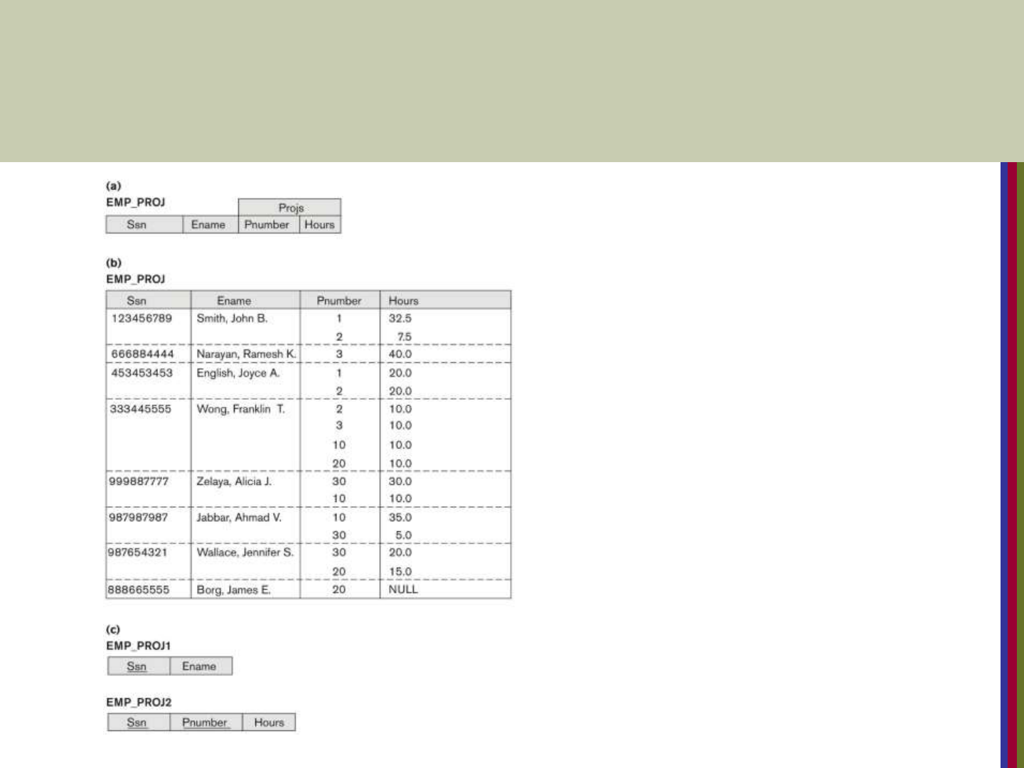
Figure 14.9 Normalization into 1NF

Slide 14- 34

Figure 14.9

Normalization into 1NF. (a)

A relation schema that is not

in 1NF. (b) Sample state of

relation DEPARTMENT. (c)

1NF version of the same

relation with redundancy.

Figure 14.10 Normalizing nested relations

into 1NF

Slide 14- 35

Figure 14.10

Normalizing nested relations into 1NF. (a) Schema of the EMP_PROJ relation with a

nested relation attribute PROJS. (b) Sample extension of the EMP_PROJ relation

showing nested relations within each tuple. (c) Decomposition of EMP_PROJ into

relations EMP_PROJ1 and EMP_PROJ2 by propagating the primary key.

3.5 Second Normal Form (1)

 Uses the concepts of FDs, primary key

 Definitions

 Prime attribute: An attribute that is member of the primary

key K

 Full functional dependency: a FD Y -> Z where removal

of any attribute from Y means the FD does not hold any

more

 Examples:

 {SSN, PNUMBER} -> HOURS is a full FD since neither SSN

-> HOURS nor PNUMBER -> HOURS hold

 {SSN, PNUMBER} -> ENAME is not a full FD (it is called a

partial dependency ) since SSN -> ENAME also holds

Slide 14- 36

Second Normal Form (2)

 A relation schema R is in second normal form

(2NF) if every non-prime attribute A in R is fully

functionally dependent on the primary key

 R can be decomposed into 2NF relations via the

process of 2NF normalization or “second

normalization”

Slide 14- 37

Figure 14.11 Normalizing into 2NF and

3NF

Slide 14- 38

Figure 14.11

Normalizing into 2NF and 3NF.

(a) Normalizing EMP_PROJ into

2NF relations. (b) Normalizing

EMP_DEPT into 3NF relations.

Figure 14.12 Normalization into 2NF and

3NF

Slide 14- 39

Figure 14.12

Normalization into 2NF

and 3NF. (a) The LOTS

relation with its

functional dependencies

FD1 through FD4.

(b) Decomposing into

the 2NF relations LOTS1

and LOTS2. (c)

Decomposing LOTS1

into the 3NF relations

LOTS1A and LOTS1B.

(d) Progressive

normalization of LOTS

into a 3NF design.

3.6 Third Normal Form (1)

 Definition:

 Transitive functional dependency: a FD X -> Z

that can be derived from two FDs X -> Y and Y ->

Z

 Examples:

 SSN -> DMGRSSN is a transitive FD

 Since SSN -> DNUMBER and DNUMBER ->

DMGRSSN hold

 SSN -> ENAME is non-transitive

 Since there is no set of attributes X where SSN -> X

and X -> ENAME

Slide 14- 40

Third Normal Form (2)

 A relation schema R is in third normal form (3NF) if it is

in 2NF and no non-prime attribute A in R is transitively

dependent on the primary key

 R can be decomposed into 3NF relations via the process

of 3NF normalization

 NOTE:

 In X -> Y and Y -> Z, with X as the primary key, we consider

this a problem only if Y is not a candidate key.

 When Y is a candidate key, there is no problem with the

transitive dependency .

 E.g., Consider EMP (SSN, Emp#, Salary ).

 Here, SSN -> Emp# -> Salary and Emp# is a candidate key.

Slide 14- 41

Normal Forms Defined Informally

 1

st

normal form

 All attributes depend on the key

 2

nd

normal form

 All attributes depend on the whole key

 3

rd

normal form

 All attributes depend on nothing but the key

Slide 14- 42

4. General Normal Form Definitions (For

Multiple Keys) (1)

 The above definitions consider the primary key

only

 The following more general definitions take into

account relations with multiple candidate keys

 Any attribute involved in a candidate key is a

prime attribute

 All other attributes are called non-prime

attributes.

Slide 14- 43

4.1 General Definition of 2NF (For

Multiple Candidate Keys)

 A relation schema R is in second normal form

(2NF) if every non-prime attribute A in R is fully

functionally dependent on every key of R

 In Figure 14.12 the FD

County_name → Tax_rate violates 2NF.

So second normalization converts LOTS into

LOTS1 (Property_id#, County_name, Lot#, Area, Price)

LOTS2 ( County_name, Tax_rate)

Slide 14- 44

4.2 General Definition of Third Normal

Form

 Definition:

 Superkey of relation schema R - a set of attributes

S of R that contains a key of R

 A relation schema R is in third normal form (3NF)

if whenever a FD X → A holds in R, then either:

 (a) X is a superkey of R, or

 (b) A is a prime attribute of R

 LOTS1 relation violates 3NF because

Area → Price ; and Area is not a superkey in

LOTS1. (see Figure 14.12).

Slide 14- 45

4.3 Interpreting the General Definition of

Third Normal Form

 Consider the 2 conditions in the Definition of 3NF:

A relation schema R is in third normal form (3NF) if

whenever a FD X → A holds in R, then either:

 (a) X is a superkey of R, or

 (b) A is a prime attribute of R

 Condition (a) catches two types of violations :

- one where a prime attribute functionally determines

a non-prime attribute. This catches 2NF violations due to

non-full functional dependencies.

-second, where a non-prime attribute functionally

determines a non-prime attribute. This catches 3NF

violations due to a transitive dependency.

Slide 14- 46

4.3 Interpreting the General Definition of

Third Normal Form (2)

 ALTERNATIVE DEFINITION of 3NF: We can restate the definition

as:

A relation schema R is in third normal form (3NF) if

every non-prime attribute in R meets both of these

conditions:

 It is fully functionally dependent on every key of R

 It is non-transitively dependent on every key of R

Note that stated this way, a relation in 3NF also meets

the requirements for 2NF.

 The condition (b) from the last slide takes care of the

dependencies that “slip through” (are allowable to) 3NF

but are “caught by” BCNF which we discuss next.

Slide 14- 47

5. BCNF (Boyce-Codd Normal Form)

 A relation schema R is in Boyce-Codd Normal Form

(BCNF) if whenever an FD X → A holds in R, then X is a

superkey of R

 Each normal form is strictly stronger than the previous

one

 Every 2NF relation is in 1NF

 Every 3NF relation is in 2NF

 Every BCNF relation is in 3NF

 There exist relations that are in 3NF but not in BCNF

 Hence BCNF is considered a stronger form of 3NF

 The goal is to have each relation in BCNF (or 3NF)

Slide 14- 48

Slide 14- 49

Figure 14.13 Boyce-Codd normal form

Figure 14.13

Boyce-Codd normal form. (a) BCNF normalization of

LOTS1A with the functional dependency FD2 being lost in

the decomposition. (b) A schematic relation with FDs; it is

in 3NF, but not in BCNF due to the f.d. C → B.

Figure 14.14 A relation TEACH that is in

3NF but not in BCNF

Slide 14- 50

Figure 14.14

A relation TEACH that is in 3NF

but not BCNF.

Achieving the BCNF by Decomposition (1)

 Two FDs exist in the relation TEACH:

 fd1: { student, course} -> instructor

 fd2: instructor -> course

 {student, course} is a candidate key for this relation and

that the dependencies shown follow the pattern in Figure

14.13 (b).

 So this relation is in 3NF but not in BCNF

 A relation NOT in BCNF should be decomposed so as to

meet this property, while possibly forgoing the

preservation of all functional dependencies in the

decomposed relations.

 (See Algorithm 15.3)

Slide 14- 51

Achieving the BCNF by Decomposition (2)

 Three possible decompositions for relation TEACH

 D1: {student, instructor} and {student, course}

 D2: {course, instructor } and {course, student}

 D3: {instructor, course } and {instructor, student} 

 All three decompositions will lose fd1.

 We have to settle for sacrificing the functional dependency

preservation. But we cannot sacrifice the non-additivity property

after decomposition.

 Out of the above three, only the 3rd decomposition will not generate

spurious tuples after join.(and hence has the non-additivity property).

 A test to determine whether a binary decomposition (decomposition

into two relations) is non-additive (lossless) is discussed under

Property NJB on the next slide. We then show how the third

decomposition above meets the property.

Slide 14- 52

Slide 14- 53

Test for checking non-additivity of Binary

Relational Decompositions

 Testing Binary Decompositions for Lossless

Join (Non-additive Join) Property

 Binary Decomposition: Decomposition of a

relation R into two relations.

 PROPERTY NJB (non-additive join test for

binary decompositions): A decomposition D =

{R1, R2} of R has the lossless join property with

respect to a set of functional dependencies F on R

if and only if either

 The f.d. ((R1 ∩ R2)  (R1- R2)) is in F

+

, or

 The f.d. ((R1 ∩ R2)  (R2 - R1)) is in F

+

.

Slide 14- 54

Test for checking non-additivity of Binary

Relational Decompositions

If you apply the NJB test to the 3

decompositions of the TEACH relation:

 D1 gives Student  Instructor or Student 

Course, none of which is true.

 D2 gives Course  Instructor or Course 

Student, none of which is true.

 However, in D3 we get Instructor  Course or

Instructor  Student.

Since Instructor  Course is indeed true, the NJB

property is satisfied and D3 is determined as a non-

additive (good) decomposition.

Slide 14-55

General Procedure for achieving BCNF

when a relation fails BCNF

Here we make use the algorithm from Chapter

15 (Algorithm 15.5):

 Let R be the relation not in BCNF, let X be a subset-of R,

and let X  A be the FD that causes a violation of BCNF.

Then R may be decomposed into two relations:

 (i) R –A and (ii) X υ A.

 If either R –A or X υ A. is not in BCNF, repeat the

process.

Note that the f.d. that violated BCNF in TEACH was Instructor Course.

Hence its BCNF decomposition would be :

(TEACH – COURSE) and (Instructor υ Course), which gives

the relations: (Instructor, Student) and (Instructor, Course) that we

obtained before in decomposition D3.

Slide 14-56

5. Multivalued Dependencies and Fourth

Normal Form (1)

Definition:

 A multivalued dependency (MVD) X —>> Y specified on relation

schema R, where X and Y are both subsets of R, specifies the

following constraint on any relation state r of R: If two tuples t

1

and

t

2

exist in r such that t

1

[X] = t

2

[X], then two tuples t

3

and t

4

should

also exist in r with the following properties, where we use Z to

denote (R 2 (X υ Y)):

 t

3

[X] = t

4

[X] = t

1

[X] = t

2

[X].

 t

3

[Y] = t

1

[Y] and t

4

[Y] = t

2

[Y].

 t

3

[Z] = t

2

[Z] and t

4

[Z] = t

1

[Z].

 An MVD X —>> Y in R is called a trivial MVD if (a) Y is a subset of

X, or (b) X υ Y = R.

Slide 14-57

Multivalued Dependencies and Fourth Normal

Form (3)

Definition:

 A relation schema R is in 4NF with respect to a set of

dependencies F (that includes functional dependencies

and multivalued dependencies) if, for every nontrivial

multivalued dependency X —>> Y in F

+

, X is a superkey

for R.

 Note: F

+

is the (complete) set of all dependencies

(functional or multivalued) that will hold in every relation

state r of R that satisfies F. It is also called the closure of

F.

Figure 14.15 Fourth and fifth normal

forms.

Slide 14- 58

Figure 14.15

Fourth and fifth normal forms. (a) The EMP relation with two MVDs: Ename –>> Pname and Ename –>>

Dname. (b) Decomposing the EMP relation into two 4NF relations EMP_PROJECTS and EMP_DEPENDENTS.

(c) The relation SUPPLY with no MVDs is in 4NF but not in 5NF if it has the JD(R1, R2, R3). (d)

Decomposing the relation SUPPLY into the 5NF relations R1, R2, R3.

Slide 14- 59

6. Join Dependencies and Fifth Normal Form

(1)

Definition:

 A join dependency (JD), denoted by JD(R

1

, R

2

, ..., R

n

),

specified on relation schema R, specifies a constraint

on the states r of R.

 The constraint states that every legal state r of R should

have a non-additive join decomposition into R

1

, R

2

, ..., R

n

;

that is, for every such r we have

 * (

R1

(r), 

R2

(r), ..., 

Rn

(r)) = r

Note: an MVD is a special case of a JD where n = 2.

 A join dependency JD(R

1

, R

2

, ..., R

n

), specified on

relation schema R, is a trivial JD if one of the relation

schemas R

i

in JD(R

1

, R

2

, ..., R

n

) is equal to R.

Slide 14- 60

Join Dependencies and Fifth Normal Form (2)

Definition:

 A relation schema R is in fifth normal form

(5NF) (or Project-Join Normal Form (PJNF))

with respect to a set F of functional, multivalued,

and join dependencies if,

 for every nontrivial join dependency JD(R

1

, R

2

, ...,

R

n

) in F

+

(that is, implied by F),

 every R

i

is a superkey of R.

 Discovering join dependencies in practical databases

with hundreds of relations is next to impossible.

Therefore, 5NF is rarely used in practice.

Chapter Summary

 Informal Design Guidelines for Relational

Databases

 Functional Dependencies (FDs)

 Normal Forms (1NF, 2NF, 3NF)Based on Primary

Keys

 General Normal Form Definitions of 2NF and 3NF

(For Multiple Keys)

 BCNF (Boyce-Codd Normal Form)

 Fourth and Fifth Normal Forms

Slide 14- 61