DNA Origami Design: A How-To Tutorial

Volume 126, Article No. 126001 (2021) https://doi.org/10.6028/jres.126.001

Journal of Research of the National Institute of Standards and Technology

How to cite this article:

Majikes JM, Liddle JA (2021) DNA Origami Design: A How-To Tutorial.

J Res Natl Inst Stan 126:126001. https://doi.org/10.6028/jres.126.001

DNA Origami Design: A How-To Tutorial

Jacob M. Majikes and J. Alexander Liddle

National Institute of Standards and Technology,

Gaithersburg, MD 20899, USA

Jacob.Majikes@nist.gov

Liddle@nist.gov

While the design and assembly of DNA origami are straightforward, its relative novelty as a nanofabrication technique means that the

tools and methods for designing new structures have not been codified as well as they have for more mature technologies, such as

integrated circuits. While design approaches cannot be truly formalized until design-property relationships are fully understood, this

document attempts to provide a step-by-step guide to designing DNA origami nanostructures using the tools available at the current

state of the art.

Key words: DNA nanofabrication; DNA origami; self-assembly.

Accepted: November 27, 2020

Published: January 8, 2021

https://doi.org/10.6028/jres.126.001

1. Introduction

Deoxyribonucleic acid (DNA) origami is a powerful approach for fabricating nanostructures with

molecular precision over length scales of approximately 100 nm. In addition, the ability to functionalize

nanoscale objects with DNA, and other attachment chemistries, means that origami can be used as a

molecular “breadboard” to organize heterogeneous collections of items such as biomolecules, carbon

nanotubes, quantum dots, gold nanoparticles, fluorophores, etc.

On completing this tutorial, readers will have learned how to apply a basic design approach for developing

DNA origami nanostructures. Since the design-property relationships of such nanostructures are still a subject of

active research, we have chosen to focus on basic concepts, rather than trying to create a comprehensive guide.

1.1 Audience

This tutorial is designed to be used by novice designers of DNA origami systems, particularly those

performing undergraduate or early graduate-level research.

1.2 Education or Skill Level

Readers of this tutorial should be familiar with the physical properties of B-DNA, single-stranded

DNA (ssDNA), and crossover junctions. In addition, once ready to create a structure for a specific

application, the designer should determine the full list of functional requirements. This list includes

answers to the following questions: What should the structure do? What specific properties are critical to

the system’s performance?

Volume 126, Article No. 126001 (2021) https://doi.org/10.6028/jres.126.001

Journal of Research of the National Institute of Standards and Technology

2 https://doi.org/10.6028/jres.126.001

1.3 Prerequisites

The designer should have either sufficient paper for manual design (not recommended) or a design

program such as cadnano [1] (all versions sufficient), nanoengineer

, Parabon inSēquio

, or equivalent.

registered account with three-dimensional (3D) structure prediction servers such as CanDo [2, 3] is also

recommended.

1.4 Tools or Equipment

Equipment includes desktop or laptop computer equipment, craft supplies for macroscale models, and

DNA nanotechnology computer-aided design (CAD) software.

1.5 Background

The sequence specificity associated with Watson-Crick-Franklin base pairing in DNA and the ability

to synthesize DNA in an arbitrary sequence [4] combine with the ease of labeling other functional

nanomaterials with DNA to make DNA an ideal molecular Lego

. It can be used to create complex

nanostructures in large quantities at low cost, and it has capabilities that are complementary to top-down

nanostructure fabrication methods. However, the design approach required to design and deploy this

molecular assembly tool is different compared to those used for established top-down assembly techniques.

The structure of B-form double-stranded DNA (dsDNA) is shown in Fig. 1. While the structure of

DNA is a surprisingly rich field of study [5], only a few properties are relevant for programmed self-

assembly [6]. These relate to the details of the lock-and-key base-pair interaction between the adenine and

thymine (A-T) and guanine and cytosine (G-C) bases in DNA polymers. Due to the asymmetry of the DNA

polymer and the shapes of the bases, canonical base pairs only form between antiparallel strands of DNA.

DNA strands can be described as antiparallel because each strand has a chemical direction, represented by

the asymmetric carbon positions (5′ and 3′) at which the phosphates are bonded to the sugar. By

convention, the start of the DNA strand is called the 5′ end, because it terminates with a phosphate at the 5′

carbon position, while the final base of the strand is called the 3′ end, because it terminates with a hydroxyl

group at the 3′ carbon position. Also, because the base-pair geometry is not symmetric, the helix has a

minor groove and a broader major groove. If a strand were to leave the helix, e.g., to make an addressable

sticky end, it would be connected to the helix at the last phosphate/sugar moiety attached to a base engaged

in the helix. As such, whether in crossovers or sticky ends, the choice of the z-axis position for a connection

to the helix determines the rotation of that position around the helix.

The principal mechanism of nanostructure fabrication using DNA relies on the ability of DNA strands to

cross over from one dsDNA helix to another adjacent helix, thereby connecting them. These “crossovers” can

be programmed to occur at specific locations using sequence design and base pairing of ssDNA strands to

create dsDNA helices. Crossovers may be formed anywhere, subject to the constraint that the phosphate

backbones are aligned. Figure 2 shows the detailed helix and schematic line representations of a DNA

crossover. One-dimensional (1D) self-assembly along the helix can be used to create both two-dimensional

(2D) and 3D structures. The reader is directed to numerous recent reviews for structure examples [7, 8].

Side-by-side comparison of crossover representations is useful because the design process occurs using

the line representation, but the rules allowing crossovers arise from physical realities visible in the helical

representation. Additionally, one should note that the crossovers shown in Fig. 2 are antiparallel. That is to

say, the yellow and green strands reverse their direction on being forced to exchange helices. While

Certain commercial items are identified in this paper in order to specify the experimental procedure adequately. Such identification

does not imply recommendation or endorsement by NIST, nor does it imply that the software, materials, or equipment identified are

necessarily the best available for the purpose.

Volume 126, Article No. 126001 (2021) https://doi.org/10.6028/jres.126.001

Journal of Research of the National Institute of Standards and Technology

3 https://doi.org/10.6028/jres.126.001

structures have been designed with parallel crossovers where the strands do not reverse [6, 9], they have not

readily been allowed by most CAD tools and represent a minority of crossovers used.

Fig 1. Structure of B-form dsDNA and major/minor grooves arising from base-pair geometry in which the sugar/phosphates split the

head-on view of the double helix into 3.6 rad (210 °) and 2.6 rad (150 °), respectively. The phosphate groups that link the sugars of

bases in the z axis are in and out of page in this illustration. The major and minor grooves here are not to scale.

Fig. 2. DNA crossover between helices. (Left) Helix representation. (Middle) Base pairing. (Right) Schematic line representation

showing antiparallel base pairing with 5′ and 3′ ends denoted by squares and triangles, respectively.

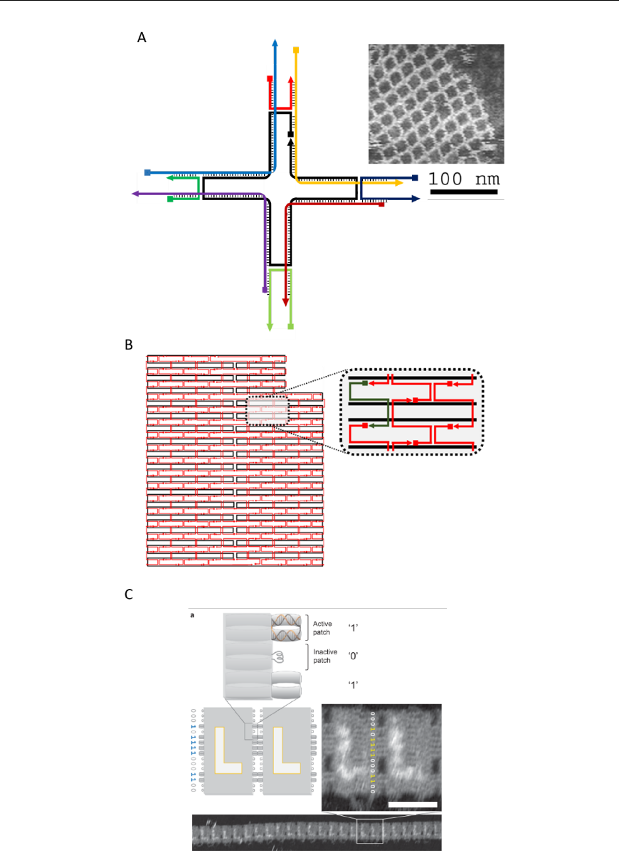
While a full review of DNA self-assembly techniques is beyond the scope of this document, we

illustrate how typical structures can be built from connected crossovers in Fig. 3. DNA tiles (Fig. 3A) often

require the fewest distinct DNA strands, and can polymerize in a variety of ways [6]. They are, however,

notoriously sensitive to design and stoichiometry, and implementation of a tile system often requires time-

consuming tuning of relative strand concentrations [6]. Developed, in part, to overcome this problem, DNA

origami (Fig. 3B) comprise a long scaffold, derived from a viral genome, held together by crossovers

programmed into synthetic ssDNA strands, or staples, with which it binds [10]. This approach allows the

staple strands to be added in excess concentration relative to the scaffold, which drives the self-assembly

Volume 126, Article No. 126001 (2021) https://doi.org/10.6028/jres.126.001

Journal of Research of the National Institute of Standards and Technology

4 https://doi.org/10.6028/jres.126.001

towards the desired structure. DNA origami systems may be designed to assemble into larger structures via

programmed interactions between multiple origami structures [11–13] (Fig. 3C).

While the fabrication of a new 3D structure can be readily accomplished without advanced background

knowledge, the design process itself is not intuitive. Fabrication of a structure by self-assembly converts

ssDNA strand sequence information into 3D topology via base pairing. However, the inverse operation

must be performed during the design process, i.e., converting a 3D structure into a linear sequence of bases.

While no individual step in the design flow is unusually difficult, an organized, iterative approach

significantly simplifies the process.

In attempting the design process, it is important to appreciate that current characterization capabilities

limit our understanding of the design-property relationships (like yield, mechanical strength, etc.). This

deficit in understanding increases the risk of failure for any one particular design and should be kept in

mind.

2. Basic Energetics, Yield, and Modeling of DNA Origami

While our understanding of the design-property relationships for many DNA nanotechnology systems

is insufficient to permit development and application of general, automated design tools (although

automated design tools that work within specific design constraints have been created [14–16]), there is a

consensus on many underpinning concepts, described here in brief. We begin with an examination of the

energetics driving the self-assembly of biological dsDNA, and we compare them with the energetics of

DNA origami. Next, we discuss the yield of the assembly process in creating the desired product. Finally,

we address common modeling and simulation tools used for these systems.

The energetics of classical dsDNA, i.e., Watson-Crick-Franklin base pairing, are predictable based on

the sequence and length of the DNA, where G-C pairings are more stable than A-T ones, resulting in a

higher melting temperature (T

) for G-C–rich sequences [17]. When dsDNA forms, the hydrophobic bases

are shielded from solution: Base-base interactions, called “base stacking,” along the long axis of the helix

are responsible for more of the favorable free energy of hybridization than the hydrogen bonding associated

with A-T and G-C base pairing.

Note: Future developments will doubtless improve our understanding of design-property trade-offs,

which are currently obscured by limited measurement capabilities.

While at this stage, many design choices are equivalent due to limited information, this document is

written in the hopes that future insights may be readily included into the design process described here.

Note: Notes will highlight considerations or pitfalls; red notes will indicate particular importance.

Volume 126, Article No. 126001 (2021) https://doi.org/10.6028/jres.126.001

Journal of Research of the National Institute of Standards and Technology

5 https://doi.org/10.6028/jres.126.001

Fig. 3. Increasing complexity in assembly. (A) DNA tile, capable of 2D polymerization, comprising four crossovers [13]. (B) Typical

2D DNA origami, containing >400 crossovers. (C) Programmed stacking between origami structures [12].

Volume 126, Article No. 126001 (2021) https://doi.org/10.6028/jres.126.001

Journal of Research of the National Institute of Standards and Technology

6 https://doi.org/10.6028/jres.126.001

The energetics of DNA origami are at least an order of magnitude more complicated than classical

dsDNA [18]. Each ssDNA strand, or staple, in an origami has multiple subsequences, allowing it to form

one or more crossovers and jump between helices. Hybridization of these subsequences can behave

independently for topologically distant staples or cooperatively for nearby staples, where each “correct”

binding event energetically reinforces nearby correct binding events [18, 19]. This cooperativity

significantly improves the quality of assembly, but it also obscures our ability to measure and understand

assembly energetics. A first form of cooperativity occurs between subsequences on the same staple. When

a first subsequence on an ssDNA strand binds to the scaffold, the other subsequences on that particular

molecule have a dramatically increased probability of colliding with, and binding to, the scaffold. This can

be equivalently described using either a unimolecular equilibrium constant including an energetic penalty

for topological effects, or a bimolecular equilibrium constant with a j-factor that represents those effects

[20–22]. These topological effects are the second relevant form of cooperativity. There is an unfavorable

energetic contribution associated with conformational entropy loss between a free scaffold and one bound

into an origami. This penalty is universal across the structure, so an individual folding event will

cooperatively reduce the penalty for its neighbors. Finally, there is interstaple base stacking. If two

subsequences end immediately adjacent to one another along the scaffold, then the ending hydrophobic

bases, which would otherwise be exposed to water, are shielded from solution [23].

As with energetics, the yield of DNA origami is a comprehensive topic, and its full scope extends

beyond this document. Yield in these systems may be defined as the number of structures that have the

correct shape in microscopy, i.e., imaging yield, or it may be defined through the total number of discrete

staple binding defects, i.e., staple yield, or it may be defined through the ratio of appropriately incorporated

functional units to imaged origami, i.e., functional yield. While staple yield is the most difficult to measure

[24], it determines the other two, and it is the most relevant to design.

Staple yield defects, as illustrated

in Fig. 4, often take the form of missing or additional unprogrammed

staples. Individual defects are often too small to detect via imaging, and they may occur in locations

irrelevant for functional yield. In the illustrated case, the red/yellow/blue strands formed together first, but

instead of correctly binding the two subsequences on a single green strand, they bound either two separate

copies of the green strand or no copies of the green strand. The desired structure and the extra-strand defect

have similar energetics because the same sequences/lengths of dsDNA are formed, with the only difference

being a loss of translational entropy in the second copy. This loss is 3/2R, where R is the gas constant, and

T is the temperature. This malformed structure would then have two unsatisfied subsequences floating in

solution, which could potentially further polymerize. Generally speaking, these defects are avoided through

careful tuning of the relative concentrations of each strand, particularly for tile-based systems [6], and

through inherent cooperativity, particularly for origami [19].

Origami also has a natural stoichiometric control in which all staples bind to a single scaffold, allowing the

staples to be added in excess, and preventing missing-strand defects. For other systems, increasing the staple

concentration would dramatically increase extra-strand defects. However, the first form of cooperativity, described

above as the transition from bimolecular to unimolecular binding, favors the first staple molecule to bind to a

scaffold, preventing extra-strand defects even at high staple excesses. This is critical, because using high excesses of

staples allows one to drive the system away from missing-strand defects. In short, origami’s natural stoichiometric

control allows for dramatically higher yield of the desired structure for significantly less experimental effort. We

recommend the following papers for those interested in more depth on this topic [18, 25–28].

A related consideration is the synthesis yield of synthetic ssDNA. Phosphoramidite DNA synthesis

adds each base in a sequence with >99 % efficiency. However, the probability of synthesizing the correct

sequence in its entirety is this efficiency raised to the power of the number of bases. It is not uncommon for

a fraction of synthesized staple strands to be missing bases. If these missing bases occur on only one

subsequence, it can guarantee an extra-strand defect. The natural stoichiometric control in origami reduces

the likelihood of this, because a fully correct strand may bind in the second extra-strand position, where

cooperative energetic effects will favor it to exchange and displace the strand with the incorrect sequence.

Volume 126, Article No. 126001 (2021) https://doi.org/10.6028/jres.126.001

Journal of Research of the National Institute of Standards and Technology

7 https://doi.org/10.6028/jres.126.001

Fig. 4. Examples of defect types for a primitive crossover.

While DNA origami assembly has been modeled and simulated, there are relatively few tools accessible

that do not require a significant investment to implement. However, simpler tools are available that provide

some useful insights. Web-based thermodynamics calculators predict classic DNA hybridization energetics

and predict unwanted hairpin formation [29–31], although these tools can typically only manage single

hybridization subsequences. CanDo is a finite element analysis tool, which treats the dsDNA helices as static

cylinders that can be torqued as they are welded together by crossovers and subject to thermal energy [32].

Finally, tools for molecular dynamics (MD), coarse graining, and multiscale modeling exist. MD simulates

behavior by treating atoms and bonds as beads and springs, respectively, with appropriate terms for

electrostatics, etc. [33–36]. MD is generally more accurate than coarse graining, which treats entire bases or

chemical subunits of bases as a single bead [37], but consumes so much more computational power that it

often cannot simulate events that occur at a timescale longer than nanoseconds. Multiscale modeling is a

technique by which different levels of coarse graining and MD are simulated and interchanged [38].

3. Common Terms

Scaffold

: Long DNA strand that is bound together to form an origami. It is often circular,

ssDNA, and sourced from a virus, although this is not always the case [39].

Scaffold routing: Raster pattern through which the scaffold travels back and forth through the structure.

Crossover: Position where DNA helices exchange ssDNA strands, linking them.

Staple: Short oligomer ssDNA sequences, usually synthetic, forcing the scaffold to route

into a desired shape.

Staple subsequence: Contiguous subset of the staple sequence that binds a contiguous sequence along

the scaffold. Subsequences are separated by crossovers.

Staple motif: Pattern of staple subsequence divisions that reoccurs throughout a structure, e.g.,

the 8 base-pair (bp) subsequence – 16 bp subsequence – 8 bp subsequence

commonly used in 2D origami such as the Rothemund Tall Rectangle [10].

Fold: The change in topology of the scaffold when a crossover, or ½ crossover, forms.

Volume 126, Article No. 126001 (2021) https://doi.org/10.6028/jres.126.001

Journal of Research of the National Institute of Standards and Technology

8 https://doi.org/10.6028/jres.126.001

Sticky end: A short subsequence left intentionally unbound at a specific position in a

structure that will later be used to bind the structure and other nanoscale objects,

including nanoparticles, biomolecules, and other structures.

4. Instructions

Design methodologies are inherently unique because of system constraints. Due to the nature of DNA synthesis,

and specifically the minimum amount of material that it is feasible to synthesize or purchase, the time and money

needed to produce a prototype structure are approximately the same as those required for large-scale purchases. This

means that the number of practicable design iterations is limited by the expense of the design-prototype-test cycle.

This tutorial attempts to apply basic engineering design theory to minimize the number of design cycles.

As noted above, our ability to reduce the number of design cycles is hampered by our ignorance of

design-property relationships, which is, in turn, exacerbated by the limited characterization capabilities

currently available. To complicate matters further, the design space for DNA nanofabrication is large. In a

very real sense, our ignorance is a meaningful constraint; without knowledge of the design-property

relationships linking the items in Fig. 5, it is common for even experienced practitioners to get trapped in

an infinite design-iteration loop, searching for a “perfect” structure, which may or may not be physically

realizable. Additionally, given the limited number of design parameters that can be varied, any attempt to

optimize one property is highly likely to dramatically change the others.

Fig. 5. Examples of properties of interest, the attributes of a structure that determine them, and the relatively few design choices that

determine those attributes in a nonorthogonal fashion.

Volume 126, Article No. 126001 (2021) https://doi.org/10.6028/jres.126.001

Journal of Research of the National Institute of Standards and Technology

9 https://doi.org/10.6028/jres.126.001

4.1 Predesign

As with almost any complex endeavor, the importance of predesign or preproduction cannot be

overstated. Given the relative immaturity of both the field of DNA nanotechnology and the nascent CAD

tool market created to serve it, the actual design process can be highly unintuitive. Beginning design

without a meaningful list of specifications invites significant loss of time.

Defining Functional Requirements:

a. List all physical features relevant to the purpose/application, such as level of control needed over

distance between specific functional components, overall footprint, accessibility of components to

solution, chirality, stimuli response, dynamic motion, inter-structure interactions, etc.

b. Determine how success in creating the desired structure will be determined.

b.I. During development:

for example, transmission electron microscope (TEM), atomic force microscopy (AFM), gel

electrophoresis.

b.II. During use:

for example, pharmaceutical activity, total number of actuation cycles before failure.

c. Order these physical features by their impact on the probability of success in application.

c.I. Combine the above information into a single set of specifications.

c.II. Add fabrication constraints, e.g., monetary constraints on number of prototyping cycles.

Two constraints that pertain to the majority of origami are the length and, commonly, the circularity of

their scaffolds, although both can be circumvented through application of production and enzymatic

methods [40]. Practically, this means that most structures are limited to a maximum of 7 249 bases,

corresponding to a dsDNA length of 2 389 nm or a surface area of approximately 5 000 nm

(6 000 nm

for

2D structures after relaxation and expansion).

The ubiquity of the most common scaffold, the M13mp18 genome, is in part historical and in part

practical. The practical considerations are as follows. The M13 bacteriophage infects the bacterium

Escherichia coli (E. coli), both of which have been researched exhaustively. The M13 bacteriophage is well

situated in inherent trade-offs among the type of virus (ssDNA, dsDNA, ssRNA, dsRNA), the length of the

viral genome, and the mutation rate [41]. While the M13 bacteriophage packages its genome as ssDNA,

which is highly desirable for origami, its packaging accommodates varying lengths of ssDNA without

significant mutation concerns. The cylindrical viral capsid consists of a handful of proteins at the caps and

a repeating coat protein along the cylinder wall. For the M13 phage, changing the amount of ssDNA

packaged can be accommodated with a change in the number of sidewall proteins and the concomitant

length of the viral capsid cylinder. The use of the mp18 sequence specifically, rather than another version

of M13, is largely historical, since it was used in Paul Rothemund’s initial work on DNA origami [10].

While longer and shorter scaffolds have been developed and employed [42, 43], the success and utility of

the original have limited the drive to explore this design variable in detail.

4.2 Macroscale Prototyping

Because true nanoscale prototypes are infeasibly expensive in both time and money, macroscale

prototyping is critical to efficient design. Mockups can be made with pen and paper, dowel rods, magnetic

toys, etc. Note: Colored magnetic bars are particularly useful for this purpose.

Note: Given our current knowledge, subjective choices are unavoidable.

Caveat Lector: Hic Sunt Dracones.

Volume 126, Article No. 126001 (2021) https://doi.org/10.6028/jres.126.001

Journal of Research of the National Institute of Standards and Technology

10 https://doi.org/10.6028/jres.126.001

Creating mockups is largely iterative, as final and initial designs are rarely identical. If at any point it is

likely that the specifications and constraints cannot be satisfied for a given structure, reiterate from the most

relevant step.

a. Build a mockup (Fig. 6).

Attributes of effective mockups include the following:

• It is easy to label and relabel subsections.

• They are easy to assemble/disassemble.

• They have rotatable joints for easier flattening.

b. Estimate whether specification is feasible.

For example, for each edge/surface of a structure, determine:

• How many helices will run through this edge/surface?

• Given the number of helices and relative proportions, can the physical specifications and the

constraint on dsDNA length be met simultaneously?

Fig. 6. Tetrahedron mockup.

c. “Flatten” the mockup (Fig. 7).

Both structure design by hand and most available CAD tools route the scaffold in 2D and force all

helices to appear as if they are parallel. It is therefore important to be able to flatten the model to

visualize the relationship between the design and the CAD representation.

Fig. 7. (Left) 3D mockup. (Right) Flattened mockup.

Note: Only check as many specifications/constraints as are relevant at each step.

Many specifications can only be estimated later when the design is more fully realized.

If specifications/constraints cannot be satisfied, try a new shape.

This step will be repeated throughout the design process.

Volume 126, Article No. 126001 (2021) https://doi.org/10.6028/jres.126.001

Journal of Research of the National Institute of Standards and Technology

11 https://doi.org/10.6028/jres.126.001

d. Identify and label the subsections and their interconnections (Fig. 8). For an additional example of

the importance of this concept, see CAD drawing in Fig. 12.

Fig. 8. (Left) Annotated, flattened mockup schematic including topological links. (Right) Flattened mockup schematic after

parallelization of helices.

e. Select the helix arrangement, also called a scaffold lattice (Fig. 9), and mock up a routing pattern (Fig. 10).

Scaffold

Lattice

Helix

Arrangement

Fig. 9. Scaffold lattice examples for honeycomb (top) and square (bottom) lattices. Dotted circles indicate potential locations for other

helices, and full cylinders indicate helices in the design.

Note:

Lattice choice will constrain later options for crossover distances/density. However, it is preferable to

make only one design choice at a time and iterate, so it is advisable to focus on accommodating the

circular nature of the scaffold and length/size constraints at this stage.

Volume 126, Article No. 126001 (2021) https://doi.org/10.6028/jres.126.001

Journal of Research of the National Institute of Standards and Technology

12 https://doi.org/10.6028/jres.126.001

Fig. 10. Physical mockup of scaffold routing using a beaded chain.

f. Using the mockup routing pattern, draw a full routing pattern (Fig. 11).

2D 3D

Scaffold Routing

Fig. 11. Example routing patterns for (left) 2D square lattice structures and (right) 3D hexagonal lattice structures.

Note:

Square lattices easily lie flat on surfaces but have difficult-to-manage internal strain (Sec. 4.5).

As a default, the square lattice is preferable for surface applications or if AFM will be the primary

imaging technique. The hexagonal lattice is typically better suited to 3D applications.

Volume 126, Article No. 126001 (2021) https://doi.org/10.6028/jres.126.001

Journal of Research of the National Institute of Standards and Technology

13 https://doi.org/10.6028/jres.126.001

g. Repeat step b—As the rough design is now more complete, confirm that specifications can be met:

• Is it physically possible to perform a valid scaffold routing given that the scaffold is circular?

• Are length/size specifications still feasible?

4.3 Computer-Aided Design (CAD)

For convenience, the cadnano2.0 [1] (cadnano.org/ & github.com/douglaslab/cadnano2) design tool

will be used as an example in this section. Other CAD tools, such as scadnano (scadnano.org/), SAMSON-

adenita toolkit [44] (www.samson-connect.net/elements.html), vHelix [45] (vhelix.net/), and Daedalus [46]

(daedalus-dna-origami.org/), are readily available and may have their own advantages. As many of these

tools are open-source tools, we used a GIT tool, GitHub desktop, to ensure operation of the most recent

version and to minimize installation problems.

Figure 12 shows two example designs and CAD screenshots. The visual complexity associated with

the routed scaffold and 200+ interconnected staples can make CAD modification difficult. Because of this,

emphasis is placed on carefully planning both the design and the CAD file to make both visualization and

modification less cumbersome. Some CAD tools allow for rotation of helices within a design (Fig. 12),

which can reduce some, but not all, visual clutter.

Note: This tutorial will only address the software aspects of initial design steps. The reader is advised

to consult user documents for their CAD tool of choice.

Note: It is impossible to avoid significant visual clutter when representing the interconnections present

in even a simple 3D structure.

Because available CAD tools can be inconvenient for arbitrary modification of designs, a minimally

cluttered design document streamlines new structure development.

The right side of Fig. 12 provides an example in which visual clutter could become problematic. If

empty helices were not placed between bundles A and F, or if the vertical placement of the bundles was

mismanaged, it would be difficult to identify individual staple locations if, for example, one wished to

label the midpoint of two bundles with unique nanoparticles.

Volume 126, Article No. 126001 (2021) https://doi.org/10.6028/jres.126.001

Journal of Research of the National Institute of Standards and Technology

14 https://doi.org/10.6028/jres.126.001

Notched Rectangle ( 2D )

Tetrahedron ( 3D )

Fig. 12. Examples of origami design and CAD screenshot. (Left) Notched rectangle structure. (Left-Top) Graphic representation of

design. (Left-Bottom) Screenshot of CAD screenshot. (Right) Tetrahedron structure. (Right-Middle) cadnano CAD screenshot.

(Right-Bottom) scadnano CAD screenshot.

h. Define the workspace (Fig. 13A–D).

h.I. Select helix type (Fig. 13A).

h.II. Define helices (Fig. 13B–C). For cadnano, the left window looks down the z axis of the helices,

while the right window has the z axis running from left to right.

h.III. When helices on the left are clicked, an “empty” helix on the right will appear.

In cadnano2.0, the helices cannot be reordered. It is advisable to add “empty” helices between

substructure units to make them visibly distinct from one another, e.g., A–F in the tetrahedron

in Fig. 12.

h.IV. Clicking again, holding, and dragging across the helices on the left will automatically generate

a scaffold routing between all the helices over which the mouse was dragged over (Fig 13D).

Note: This step must often be reiterated to ensure the CAD workspace is easily legible.

Volume 126, Article No. 126001 (2021) https://doi.org/10.6028/jres.126.001

Journal of Research of the National Institute of Standards and Technology

15 https://doi.org/10.6028/jres.126.001

Fig. 13. (A-D) CAD images corresponding to step h. (A) Lattice selection determining staking of helices when looking down the z

axis. (B) Selection of helices to populate into CAD file. (C) Populated helices for a six-helix bundle. (D) Automatic scaffold routing

created by dragging mouse across helices in C.

Note: cadnano v2.0 centers the new routing around the yellow slider in the right window.

Note: Any CAD tool will automatically track potential crossover spacings for both the scaffold and

staples given the properties of B-DNA and the positions of neighboring helices.

Volume 126, Article No. 126001 (2021) https://doi.org/10.6028/jres.126.001

Journal of Research of the National Institute of Standards and Technology

16 https://doi.org/10.6028/jres.126.001

i. Test staple motifs on a small section of the scaffold routing pattern. For examples, see Fig. 14.

i.I. The goal, at this step, is to confirm that a valid staple motif exists for the chosen scaffold routing

that can meet the design specifications and constraints.

i.II. Staples may be drawn manually, or they may be edited after generation via cadnano’s

“autostaple” function.

o Consider the following criteria when evaluating staple motifs and design specifications.

 Consider the staple fit over the scaffold “seams,” because positions where the scaffold crosses

over between helices are typically the longest distance folds, and the most susceptible to

defect formation:

o Fewer than 5–8 bases of connection may not have desired stability.

 Consider the distance between, and number of, crossovers:

o More crossovers => stiffer structure (along crossover axis).

o More crossovers => more internal strain (addressed in initial testing and fine tuning).

 Consider the 5′ and 3′ (start and stop) position locations that are natural locations to extend

sticky ends and create functional binding sites (addressed in additional conceptual tools

section).

Note: cadnano v2.0 indicates the rotational position of the scaffold bases at each helix underneath the

yellow slider as a blue line on the helix in the left window, Fig. 13D).

The blue line indicates the position of the minor groove, where strands exit/enter the helix. A more

general description is given in Sec.5.3.

Visual Clutter Management Checklist

In current software versions, the helix positions on the right window cannot be modified. Care should

be taken with their arrangement to minimize visual clutter.

We advise the following approach.

Visual proximity on the right window schematic is dependent on the order in which the helices are

activated, step h, on the left window. To minimize visual clutter, the helices should be activated in an

order that groups substructures.

1. Identify the number of substructure sections in the mockup.

a. Notched Rectangle = 1 substructure (Fig. 12).

b. Tetrahedron = 6 substructures (Fig. 12).

c. Tower = 5 substructures (Fig. 18).

2. For each substructure, count necessary helices and identify helices/positions where strands

will jump to other substructures (Fig. 8).

3. Label mockup substructures in an order that shortens intersubstructure connections in

flattened/parallel view.

4. Label helix order within substructures to place intersubstructure connections at the top/bottom

of that substructure in the flattened/parallel view.

5. Starting with the first substructure, activate helices in order.

6. Between substructures, activate at least two helices to provide visual space between them

7. Click/fill helices, step h.III, in the same order as above.

a. If the automatically filled scaffold is unsatisfactory, then it is advisable to undo the

action, move the yellow slider that centers the automatic filling function, and try

again before resorting to manual drawing tools.

8. SAVE all intermediate drafts as separate files.

Note: It is not possible to represent a 3D structure as a flattened and parallel line schematic without

crossovers running “over” the rest of the design. While no arrangement will prevent problematic visual

clutter, CAD workspace organization can significantly reduce it.

Volume 126, Article No. 126001 (2021) https://doi.org/10.6028/jres.126.001

Journal of Research of the National Institute of Standards and Technology

17 https://doi.org/10.6028/jres.126.001

Fig. 14. Example staple motifs on the square 2D lattice, with tentative naming convention based on the number of bases in each

subsequence with differentiation for full and half crossovers where necessary.

j. For testing, we advise the following steps (Fig. 15).

j.I. Confirm the autostaple pattern has satisfactory crossover options; if not, then delete and recenter

the scaffold routing (Fig. 15A).

j.II. Treat the scaffold seam regions separately from the rest of the structure.

j.III. Identify a staple motif rule, e.g., one 8 base subsequence, one 16 base subsequence, and one 8

base subsequence, preferably with a nucleating subsequence [47].

k. Save a copy of the scaffold routing empty of staples (Fig. 16).

l. Attempt to tile selected motif over a small area. Write down or otherwise confirm the tentative pattern

of the staple motif.

m. Estimate feasibility of meeting specifications in step b.

n. Populate the routing pattern with the tentative staple motif choice from step j.III. An example of this is

shown in Fig. 12.

o. Save the completed file under a new file name.

Note: Synthetic ssDNA synthesis is typically limited to <60 to 100 bases.

The yield of a synthetic ssDNA is roughly equal to 0.95

to 0.99

, where N is the number of bases.

Long staples have lower yield but theoretically allow higher thermal stability because longer DNA

domains melt at higher temperatures.

Note: Staple motifs, particularly for multilayer 3D objects, are one of the few choices for which there is

a known failure mode. Staple motifs consisting only of equal-length subsequences have a failure in 3D,

honeycomb lattice structures and have been known to result in failed annealing and aggregation.

Where possible, staples should be designed with a “nucleating” subsequence of longer length [47].

Volume 126, Article No. 126001 (2021) https://doi.org/10.6028/jres.126.001

Journal of Research of the National Institute of Standards and Technology

18 https://doi.org/10.6028/jres.126.001

Fig. 15. Example tests for staple motifs. (A) Initial scaffold routing. (B) Staple crossover pattern generated by the autostaple function.

(C) Incremental division of the staple crossover pattern into individual staples of a length that can be ordered for custom synthesis.

Volume 126, Article No. 126001 (2021) https://doi.org/10.6028/jres.126.001

Journal of Research of the National Institute of Standards and Technology

19 https://doi.org/10.6028/jres.126.001

Notched Rectangle ( 2D )

Tetrahedron ( 3D )

Fig. 16. Example routing maps and final staple screenshots matching Fig. 12.

Note: Step n often reveals flaws in the staple motif choice or scaffold routing. Expect one or two

reiterations at this stage.

Create backup files for each staple motif and routing choice.

Volume 126, Article No. 126001 (2021) https://doi.org/10.6028/jres.126.001

Journal of Research of the National Institute of Standards and Technology

20 https://doi.org/10.6028/jres.126.001

4.4 Initial Structure Prediction

Numerous tools exist for evaluation of structures. While we use CanDo (https://cando-dna-

origami.org/), other tools, such as circleMap (https://nanohub.org/resources/cadnanovis) and University of

Illinois at Urbana–Champaign (UIUC) multiscale (http://bionano.physics.illinois.edu/origami-structure),

also exist. Physics-based simulations such as UIUC multiscale or oxDNA [37] may provide more nuanced

predictions at the cost of time and expertise to initiate. An advisable first step is to test new structures with

a finite element analysis tool such as CanDo. Finite element analysis treats each helix as an independent

cylinder and the crossovers as welds with nominally realistic levels of torque and strain given the angle of

the crossover and physical properties of DNA. Finite element analysis provides a preliminary confirmation

of the 3D structure, and it is preferable to performing an MD, coarse-grained, or multiscale modeling

simulation on the structure, which could potentially waste significant computational resources.

If curvature of the structure is irrelevant to the design specifications, then the need for testing and fine

tuning may be limited. Figure 17 shows the CanDo simulations on the notched rectangle and an AFM

image thereof. The curvature in this CanDo simulation is a reasonable representation of the effects of

internal strain and torque on 2D origami structures [48]. A 3D tower structure on the square lattice is shown

in Fig. 18.

For CanDo, red indicates a section of the structure that is freer to move, while blue indicates a static

section. CAD modification at this stage is highly dependent on design specifications. One common

modification, strain compensation for square lattice structures, will be addressed in the next section.

Fig. 17. Notched rectangle design, CanDo result, and AFM image.

Note: Finite element analysis is sufficient to predict general shape and requires minimal computing

resources. If it is necessary to perform MD or multiscale modeling for a more detailed representation

of the structure, it is advisable to wait until after the user is satisfied with the structure’s performance

in finite element analysis modeling.

Volume 126, Article No. 126001 (2021) https://doi.org/10.6028/jres.126.001

Journal of Research of the National Institute of Standards and Technology

21 https://doi.org/10.6028/jres.126.001

Fig. 18. Tower origami CanDo result.

4.5 Crossovers and Internal Strain

When addressing internal stress, strain, and torque of DNA origami, it is doubly important to know in

advance which functional requirements one is pursuing. While the interplay among design, stress, strain,

and torque is relatively easy to model, they are often difficult to visualize and implement. As a result, it is

easy to waste significant time and effort modifying these factors to no positive effect.

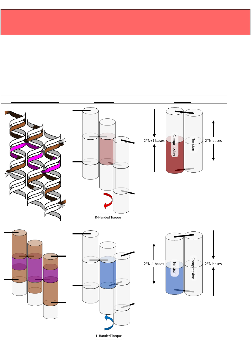
Internal strain and torque in DNA origami are well described by the analogy of welding together

springs, as illustrated in Fig. 19, where the metal of the spring represents the minor groove. In this analogy,

there are two springs that must be joined at two positions to create a larger structure. Both springs have the

same helicity and period. After the first weld, the springs are aligned, and there is a visible periodicity

where the metal of each spring touches. At these positions, one could apply a second weld with no tension

or torque. However, if one wished to weld at two positions of equal distance to the first weld, but a little

before or after this period, one would have to tighten or loosen the spring to bring those points into line.

Similarly, if one wished to weld the springs at slightly different lengths, one would simultaneously have to

compress and tighten one spring while stretching and unwinding the other.

Fig. 19. Spring analogy for over- and underwinding of DNA when helices are connected by crossovers. L-handed and R-handed

indicate left-handed and right-handed, respectively.

Volume 126, Article No. 126001 (2021) https://doi.org/10.6028/jres.126.001

Journal of Research of the National Institute of Standards and Technology

22 https://doi.org/10.6028/jres.126.001

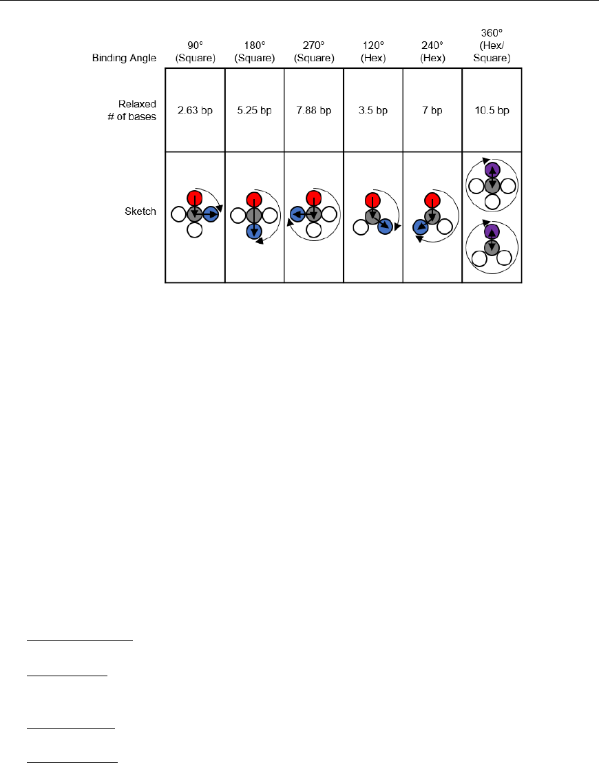
The spring analogy is imperfect, DNA cannot be treated as continuous, and crossovers can only occur

between integer numbers of bases. This can be problematic because the dsDNA helix has 10.5 bases per

full turn. The number of bases between potentially relaxed crossover positions depends on the angle

between helices being welded (Fig. 23), which can confuse the process of choosing the number of bases

between crossovers for a particular design. Binding numerous helices at a variety of angles is much more

complex than simply welding two springs.

Relaxed/Example

Torque

Strain

Fig. 20. (Left) Cylinder representation of dsDNA between crossovers. (Middle) Resulting torque within a structure if only the center

purple helix/cylinder from the left side is overwound or underwound. (Right) Schematic of strain in DNA crossovers. Torque and

strain will occur simultaneously in most systems as the sum of small contributions from all crossovers. They are depicted here as

independent for illustrative purposes only. As in Fig. 19, red indicates overwound helices, and blue indicates underwound helices.

Note: Modification/control of torque and strain in DNA nanostructures can be very time-consuming.

Before attempting to modify a structure, take time to confirm that it is necessary for your functional

specifications.

Volume 126, Article No. 126001 (2021) https://doi.org/10.6028/jres.126.001

Journal of Research of the National Institute of Standards and Technology

23 https://doi.org/10.6028/jres.126.001

The torques and compressive/tensile forces may be controlled by varying the number of bases between

crossovers (in cadnano v2.0, by using the skip and insert tools). The effects of these approaches are shown

schematically in Fig. 20 and Fig. 21. Additionally, Fig. 22 uses a full origami CAD example.

The constraints on staple length dictated by yield in ssDNA synthesis and specifications for flexibility

(requiring more/fewer crossovers) are important to consider because torque and strain are controlled via

changing crossover spacing with skips and inserts. The default spacing is a set number of bases in the

software for each lattice/angle between helices. This number must be an integer, but the relaxed number of

bases for that angle is often not an integer. A skip, when placed between crossovers, informs the software

to have one base fewer than the default between those crossovers. An insert informs the software to have

one base more than the default.

Fig. 21. (Left) Arrangement of strained/torqued helices. (Right) Approximate effect on overall structure conformation of that

strain/torque arrangement. As in Fig. 19, red indicates overwound helices, and blue indicates underwound helices.

Volume 126, Article No. 126001 (2021) https://doi.org/10.6028/jres.126.001

Journal of Research of the National Institute of Standards and Technology

24 https://doi.org/10.6028/jres.126.001

Twist

Schematic

Average

Twist

Values

Default Length:

slightly overwound

10.66 bp/turn

33.75°/bp

Alternating Skips:

10.333 bp/turn

34.84°/bp

¼ Skips:

10.5 bp/turn

34.28°/bp

¼ Skips staggered:

10.5 bp/turn

34.28°/bp

CanDo

Prediction

Fig. 22. CanDo example of DNA skips and strain compensation on a square lattice for a planar origami. The top row shows the

handedness of the torque as determined by the presence and location of skips. Red indicates right-handed torque helices, and blue

indicates left-handed torque in the twist schematic. The average twist values are indicated for each of the four designs. As noted in the

text, the number of base pairs per turn in an unstrained dsDNA helix is 10.5. The bottom row shows the outputs of the corresponding

CanDo models. These illustrate the approximate shape and local helix mobility.

The “relaxed” number of bases between crossovers depends on the enforced angle between helices, as

shown in Fig. 23. While this may be a useful reference, it is a worthwhile exercise to independently derive

these numbers. On the hexagonal lattice, the relaxed number is either an integer or ± 0.5 bases. While the

square lattice lies flat for easier AFM imaging, compensation of residual strain/torque is much easier for the

hexagonal lattice.

The reader is advised to save backup copies of the CAD file between modification attempts, and to

regularly use finite element analysis prediction for each step to ensure specifications can be met. Given the

number of files generated, a rational file naming and organizing scheme is essential.

Volume 126, Article No. 126001 (2021) https://doi.org/10.6028/jres.126.001

Journal of Research of the National Institute of Standards and Technology

25 https://doi.org/10.6028/jres.126.001

Fig. 23. Relaxed number of bases for common helix binding angles. If the distance between two crossovers is greater than a full turn,

to determine whether it is over- or underwound, subtract the largest integer multiple of 10.5 bases possible without resulting in a

negative number.

Note: Use of this strain to generate curved surfaces is addressed in Ref. [49].

5. Additional Conceptual Tools

5.1 Folding Information and its Representation

A common concern for designers of DNA origami systems is, among the multiplicity of design

options, how to determine if one is better or worse than others. Current understanding is insufficient to

answer this question, but a few conceptual tools can illustrate how structures are different.

One factor that is known to be important in origami folding are entropic penalties, which occur when

the topology of the scaffold is forced to change via staple binding. The total entropic cost of transforming

the flexible ssDNA scaffold into a single relatively inflexible block is small compared to the energy gains

associated with binding. However, this cost is levied unevenly, and it significantly discourages long-

distance folds from occurring until other staples reduce that distance. Fold distances may be visualized

within the routing pattern, circle plots, histograms, and square plots.

The routing pattern

, discussed in the instructions, conveys the desired shape of a structure and is a

central focus of the design process.

The circle plot illustrates the initial distance each fold must bridge. In the circle plot, the scaffold is

represented by the outside circle, while each arc indicates a fold. One limitation of the circle plot is that the

vast majority of folds are too small to see clearly.

Histogram plots of fold distances readily depict small folds and can be used to determine fold-distance

statistics, but they contain no information on fold nesting.

The square plots that we have devised, and that we present here for the first time, attempt to combine

the most useful aspects of circle plots and fold histograms. The scaffold in the square plot is represented by

the x axis, and in the case of a circular scaffold, it should be noted that that origin and the furthest extent

represent adjacent points on that scaffold. Folds are plotted as lines between their start/stop positions, with

the y-axis position corresponding to the initial fold distance, equal to the difference between the start and

stop positions on the scaffold for that fold. Folds plotted above/below each other will directly reduce the

looping entropy penalties for each other. In this way, cones that run from the top to bottom of the square

plot indicate folding pathways along which a long stretch of scaffold is “zipped” closed. To emphasize this

Volume 126, Article No. 126001 (2021) https://doi.org/10.6028/jres.126.001

Journal of Research of the National Institute of Standards and Technology

26 https://doi.org/10.6028/jres.126.001

feature, a transparent shading was applied from each fold down to the bottom of the plot. Darker regions

reflect many nested folds on top of one another. In short, darker shading regions imply a folding “pathway”

in which some shorter folds must occur first to enable subsequent folds.

5.2 Congruent Shapes of Various Scaffold Routing

To illustrate the plots described in Sec. 5.1 and the plethora of design choices, we created four different

DNA origami of identical, or nearly identical, 2D footprint. In an AFM or TEM, these structures would be

difficult to distinguish from one another.

The two designs most typical of 2D origami to date are the vertical and horizontal designs (Fig. 24).

The scaffold routing for these two designs places a seam that bisects the rectangular footprint along a

cardinal axis. As the rectangle has a high aspect ratio, this results in very different loop distributions. The

vertical origami has a very large number of short-fold-distance nucleating sites, but many more long-

distance folds as the system zips up the seam. In contrast, the horizontal origami has relatively few very

long or very short folds, and a large number of medium-distance folds.

The other two designs presented here are less typical but represent conceptually simple modifications

to the horizontal design. The horizontal interdigitated design moves the scaffold crossovers of the seam

back and forth so that they are no longer contiguous, broadening the distribution of fold distances. The

woven structure is the result of taking each crossover position and, if possible, having the scaffold jump

between helices rather than the staple.

In evaluating a design, we recommend use of the circle plot to confirm the number and symmetry of

substructural units in the origami, as the circle plot can be visualized on “top” of the routing for

troubleshooting. A drawback of the circle plot, shown in Fig. 25, is that it poorly depicts the very short

folds, which often comprise the majority of a structure. The square plot is more useful for identifying the

degree to which folds will occur in parallel or via a few path-dependent “zippering” interactions.

The examples in Fig. 24 illustrate design differences in cases where numerous designs occupy the

same footprint. Note: The routing patterns, particularly for the vertical origami, are not to scale.

The “horizontal” origami has helices running parallel to its long side and a central seam, and it would

be rigid in the long direction but flexible along the short direction. If one only looked at the routing map, it

would be easy to believe this origami has the greatest number of long folds because the scaffold has the

fewest turns.

The “vertical” origami has helices running parallel to its short side and a long central seam, and it

would be flexible in the long direction but rigid in the short direction. Because there are many positions

where the scaffold routes back and forth in the short direction, there are large numbers of short folds,

shown in the histogram.

The “interdigitated horizontal” origami illustrates how the fold distances in the horizontal origami

would change if the seams were shifted/interdigitated. This example shows how simple changes to the

routing pattern can dramatically change the distribution of loop distances.

Finally, the “woven” origami takes the horizontal origami design and maximizes the number of

positions where the scaffold is jumping between helices, rather than the staples.

While different routing patterns result in quite different fold distance distributions, we do not yet know

if those differences have a significant impact on the quality of self-assembly.

Volume 126, Article No. 126001 (2021) https://doi.org/10.6028/jres.126.001

Journal of Research of the National Institute of Standards and Technology

27 https://doi.org/10.6028/jres.126.001

Fig. 24. Example representation of congruent designs. For each design, Top-Left: scaffold routing, Top-Right: histogram, Bottom-

Left: circle plot, Bottom-Right: square plot.

Horizontal Origami

Horizontal Origami Interdigitated

100

0 1000 2000 3000

100

150

Counts

Fold Distance

Cumulative Percent

100

0 1000 2000 3000

100

150

Counts

Fold Distance

Cumulative Percent

Volume 126, Article No. 126001 (2021) https://doi.org/10.6028/jres.126.001

Journal of Research of the National Institute of Standards and Technology

28 https://doi.org/10.6028/jres.126.001

Fig. 24. Example representation of congruent designs. For each design, Top-Left: scaffold routing, Top-Right: histogram, Bottom-

Left: circle plot, Bottom-Right: square plot (continued).

Woven Horizontal Origami

Vertical Origami

100

0 1000 2000 3000

100

150

Counts

Fold Distance

Cumulative Percent

100

0 1000 2000 3000

100

150

Counts

Fold Distance

Cumulative Percent

Volume 126, Article No. 126001 (2021) https://doi.org/10.6028/jres.126.001

Journal of Research of the National Institute of Standards and Technology

29 https://doi.org/10.6028/jres.126.001

Fig 25. Zoom-in of respective circle plots illustrating the short folds, which can be difficult to see in circle plots.

5.3 Staple Extensions for Addressing Functional Units

Sticky ends—short lengths of unbound ssDNA—are used to create addressable sites on the origami to

which functional units such as nanoparticles or biomolecules may be added. These sticky ends may be

incorporated as a hairpin in the center of a staple or as an extension at either end of the staple. In both

cases, it is critical to know which direction relative to the bulk of the origami the sticky end will exit.

As briefly mentioned in the introductory material, the extension will exit the helix based on the

position of the minor groove at the relevant base position (Fig. 1 and Fig. 2).

This process is illustrated in Fig. 26. The simplest visualization comes from combining the direction of

the staple, the direction of the nearest crossover, and the helicity of dsDNA to determine the exit direction for

the sticky end via the right-hand rule. This can be done by imaging the right-hand-thumb in the 5′→ 3′

direction and the index finger initially in the direction of the crossover. As the hand moves along the dsDNA,

the fingers should curl at ≈ 34.3°/base in the 3′ direction. This is approximately 270° per every 8 bases.

Fig. 26. Design example and application of the right-hand rule in placing an addressable sticky end.

Volume 126, Article No. 126001 (2021) https://doi.org/10.6028/jres.126.001

Journal of Research of the National Institute of Standards and Technology

30 https://doi.org/10.6028/jres.126.001

One useful exercise is to examine the Rothemund Tall Rectangle [10], which is the basis structure for

the notched rectangle shown throughout this text. The Tall Rectangle is often used as a representative 2D

structure. Based on its design, all its 5′ and 3′ staple ends exit the origami on the same face. If functional

components are needed on both sides of the structure, a minor redesign of the staples is necessary.

Confirming this property, and attempting said staple redesigns, is a worthwhile exercise for designers

new to DNA origami.

5.4 Programmed and Unintentional Intra-origami Base Stacking

In the introduction, origami were described as being built from dsDNA helices welded together by

crossovers. There is an additional critical feature of these helices relevant to DNA origami. While the radial

surface of the helix comprises the negatively charged hydrophilic backbone, the end caps comprise the

hydrophobic bases. The sides of an origami parallel to the helix direction are hydrophilic, while those

perpendicular to the helix direction (with exposed cylinder ends) are hydrophobic.

As such, the exposed cylinder ends at the edges of DNA nanostructures are prone to reversible, low-

energy stacking [12], as shown in Fig. 27.

This stacking can be beneficial, e.g., for surface tiling, or disadvantageous, because it may lead to

uncontrolled agglomeration. A tried-and-tested of way to prevent stacking is to place a 4+ base poly-T loop

on the staples when they jump between helices at the cylinder ends. If G-C hairpins are placed in these

positions on the staples, they can create physical lock-and-key arrangements that only allow stacking

between preprogrammed substructures.

Fig. 27. Interorigami base stacking between helix ends, prevention thereof, and programmed base stacking.

5.5 Ordering and Naming Conventions

Most DNA nanofabrication CAD tools have a primary export format of comma-separated value, or

.csv, files. This is because most oligonucleotide synthesis companies perform bulk orders through .csv

Volume 126, Article No. 126001 (2021) https://doi.org/10.6028/jres.126.001

Journal of Research of the National Institute of Standards and Technology

31 https://doi.org/10.6028/jres.126.001

workbook files. While the relevant cells from the .csv file can be copied directly into the order forms, it is

advisable to take additional time to consider naming conventions.

One DNA origami typically requires 250 staple strands or more, requiring procurement of three 96

deep-well plates, with numerous individual tubes for functionalized staples. Given that one set of plates can

last for both a considerable time and for a considerable number of experiments, a consistent naming

convention is useful.

CAD tool .csv export files will typically include information such as the helix number and base

position along that helix for each staple. It is advisable to use this information as part of the name in

purchasing, to minimize frustration in future attempts to add or remove individual staples.

Toward this end, common text extraction and concatenation tools in workbook programs are useful.

Examples include LEFT() and “&” in Excel

. Combining these with an autofill function can allow for

complex names to be quickly generated for all strands. It is advisable to include properties like a structure

name abbreviation, substructure, and helix/base position of the staple.

Default mass ordering spreadsheets will often name the plates “Sheet1” to “SheetN” or “Plate1” to

“PlateN.” The wise researcher will avoid a freezer full of many structures each with multiple plates labeled

with such generic names.

6. Summary

By breaking the design process for DNA origami into a sequence of iterative operations involving

straightforward decisions and prioritizations, it is possible to streamline the creation of a new design, both

minimizing nonproductive tinkering and reducing the likelihood of errors. The general flow of this process

is applicable to other types of DNA nanofabrication systems such as single-strand tiles (SSTs) and

infinitely tiling systems.

If only one piece of advice from this document is retained by the reader, we strongly suggest that it be

the understanding that critical and intentional predesign, including the generation of a complete list of

functional requirements, is absolutely necessary to the efficient development of a working structure.

Acknowledgments

The authors would like to acknowledge Nicole Estrich for providing the 3D tetrahedron origami as

well as for useful discussions on the design process.

Contact Information

Jacob Majikes, research scientist, Microsystems and Nanotechnology Division, Physical Measurement

Laboratory, NIST, Jacob.majikes@nist.gov.

Note: As one set of origami plates can last for an extended period, it is reasonable to assume

that another researcher will have to use your notation to understand the structure.

Pay it forward by using a clear and consistent naming convention for the plates & strands.

Note: Using the helix number and base position, or other identifying feature in your CAD tool

of choice, in a naming convention will allow you or your successor to easily find and replace

individual staples for subsequent experiments/sticky strand labeling.

Volume 126, Article No. 126001 (2021) https://doi.org/10.6028/jres.126.001

Journal of Research of the National Institute of Standards and Technology

32 https://doi.org/10.6028/jres.126.001

7. References

[1] Douglas SM, Marblestone AH, Teerapittayanon S, Vazquez A, Church GM, Shih WM (2009) Rapid prototyping of 3D

DNA-origami shapes with caDNAno. Nucleic Acids Research 37(15):5001–5006.

[2] Castro CE, Kilchherr F, Kim D, Shiao EL, Wauer T, Wortmann P, Bathe M, Dietz H (2011) A primer to scaffolded DNA

origami. Nature Methods 8(3):221–229. https://doi.org/10.1038/NMETH.1570

[3] Kim D, Kilchherr F, Dietz H, Bathe M (2011) Quantitative prediction of 3D solution shape and flexibility of nucleic acid

nanostructures. Nucleic Acids Research 1(7):1–7. https://doi.org/10.1093/nar/gkr1173

[4] Carlson R (2009) The changing economics of DNA synthesis. Nature Biotechnology 27(12):1091–4.

https://doi.org/10.1038/nbt1209-1091

[5] Bloomfield VA, Crothers DM, Tinoco I (2000) Nucleic Acids: Structures, Properties, and Functions ed Stiefel J (University

Science Books, Sausalito, CA 94965).

[6] Seeman NC (2016) Structural DNA Nanotechnology (Cambridge University Press, Cambridge).

https://doi.org/10.1017/CBO9781139015516

[7] Chandrasekaran AR, Punnoose JA, Zhou L, Dey P, Dey BK, Halvorsen K (2019) DNA nanotechnology approaches for

microRNA detection and diagnosis. Nucleic Acids Research 47(20):10489–10505. https://doi.org/10.1093/nar/gkz580

[8] Ke Y, Castro C, Choi JH (2018) Structural DNA Nanotechnology : Artificial Nanostructures for Biomedical. 375–403.

[9] Shen Z, Yan H, Wang T, Seeman NC (2004) Paranemic crossover DNA: a generalized Holliday structure with applications

in nanotechnology. Journal of the American Chemical Society 126(6):1666–74. https://doi.org/10.1021/ja038381e

[10] Rothemund PWK (2006) Folding DNA to create nanoscale shapes and patterns. Nature 440(7082):297–302.

https://doi.org/10.1038/nature04586

[11] Woo S, Rothemund PWK (2014) Self-assembly of two-dimensional DNA origami lattices using cation-controlled surface

diffusion. Nature Communications 5:4889. https://doi.org/10.1038/ncomms5889

[12] Woo S, Rothemund PWK (2011) Programmable molecular recognition based on the geometry of DNA nanostructures.

Nature Chemistry 3(8):620–7. https://doi.org/10.1038/nchem.1070

[13] Strong M (2004) Protein Nanomachines. PLOS Biology 2(3). https://doi.org/10.1371/journal.pbio.0020073

[14] Jun H, Shepherd TR, Zhang K, Bricker WP, Li S, Chiu W, Bathe M (2019) Automated sequence design of 3D polyhedral

wireframe DNA origami with honeycomb edges. ACS Nano 13(2):2083–2093. https://doi.org/10.1021/acsnano.8b08671

[15] Jun H, Wang X, Bricker WP, Bathe M (2019) Automated sequence design of 2D wireframe DNA origami with honeycomb

edges. Nature Communications 10(1):1–9. https://doi.org/10.1038/s41467-019-13457-y

[16] Jun H, Zhang F, Shepherd T, Ratanalert S, Qi X, Yan H, Bathe M (2019) Autonomously designed free-form 2D DNA

origami. Science Advances 5(1):1–9. https://doi.org/10.1126/sciadv.aav0655

[17] SantaLucia J, Hicks D (2004) The thermodynamics of DNA structural motifs. Annual Review of Biophysics and

Biomolecular Structure 33:415–440. https://doi.org/10.1146/annurev.biophys.32.110601.141800

[18] Dannenberg F, Dunn KE, Bath J, Turberfield AJ, Ouldridge TE, Kwiatkowska M, Turberfield AJ, Ouldridge TE (2015)

Modelling DNA origami self-assembly at the domain level. The Journal of Chemical Physics 143(16):1–19.

https://doi.org/10.1063/1.4933426

[19] Arbona J-M, Aimé J-P, Elezgaray J (2013) Cooperativity in the annealing of DNA origamis. The Journal of Chemical

Physics 138(1):015105. https://doi.org/10.1063/1.4773405

[20] Crothers DM, Drak J, Kahn JD, Levene SDBT-M in E (1992) DNA bending, flexibility, and helical repeat by cyclization

kinetics. DNA Structures Part B: Chemical and Electrophoretic Analysis of DNA (Academic Press), Vol. 212, pp 3–29.

https://doi.org/10.1016/0076-6879(92)12003-9

[21] Jacobson H, Stockmayer WH (1950) Intramolecular Reaction in Polycondensations. I. The Theory of Linear Systems. The

Journal of Chemical Physics 1600(18). https://doi.org/10.1063/1.1747547

[22] Zhang Y, Mcewen AE, Crothers DM, Levene SD (2006) Statistical-Mechanical Theory of DNA Looping. Biophysical

Journal 90(March):1903–1912. https://doi.org/10.1529/biophysj.105.070490

[23] Yakovchuk P, Protozanova E, Frank-Kamenetskii MD (2006) Base-stacking and base-pairing contributions into thermal

stability of the DNA double helix. Nucleic Acids Research 34(2):564–574. https://doi.org/10.1093/nar/gkj454

[24] Strauss MT, Schueder F, Haas D, Nickels PC, Jungmann R (2018) Quantifying absolute addressability in DNA origami with

molecular resolution. Nature Communications 9(1):1–7.

https://doi.org/10.1038/s41467-018-04031-z

[25] Lee Tin Wah J, David C, Rudiuk S, Baigl D, Estevez-Torres AAA, Wah JLT, David C, Rudiuk S, Baigl D, Estevez-Torres

AAA (2016) Observing and Controlling the Folding Pathway of DNA Origami at the Nanoscale. ACS Nano 10(2):1978–

1987. https://doi.org/10.1021/acsnano.5b05972

[26] Jacobs WM, Reinhardt A, Frenkel D (2015) Rational design of self-assembly pathways for complex multicomponent

structures. Proceedings of the National Academy of Sciences of the United States of America 112(20):6313–8.

https://doi.org/10.1073/pnas.1502210112

[27] Dunn KE, Dannenberg F, Ouldridge TE, Kwiatkowska M, Turberfield AJ, Bath J (2015) Guiding the folding pathway of

DNA origami. Nature. https://doi.org/10.1038/nature14860

[28] Wei X, Nangreave J, Liu Y (2014) Uncovering the self-assembly of DNA nanostructures by thermodynamics and kinetics.

Accounts of Chemical Research 47(6):1861–1870. https://doi.org/10.1021/ar5000665

[29] Owczarzy R, Tataurov A V., Wu Y, Manthey JA, McQuisten KA, Almabrazi HG, Pedersen KF, Lin Y, Garretson J,

McEntaggart NO, Sailor CA, Dawson RB, Peek AS (2008) IDT SciTools: a suite for analysis and design of nucleic acid

oligomers. Nucleic Acids Research 36(Web Server issue):W163-9. https://doi.org/10.1093/nar/gkn198

[30] Kibbe WA (2007) OligoCalc: an online oligonucleotide properties calculator. Nucleic Acids Research 35(Web Server

issue):W43-6. https://doi.org/10.1093/nar/gkm234

[31] Tulpan D, Andronescu M, Leger S (2010) Free energy estimation of short DNA duplex hybridizations. BMC Bioinformatics

11. https://doi.org/10.1186/1471-2105-11-105

Volume 126, Article No. 126001 (2021) https://doi.org/10.6028/jres.126.001

Journal of Research of the National Institute of Standards and Technology

33 https://doi.org/10.6028/jres.126.001

[32] Kim DN, Kilchherr F, Dietz H, Bathe M (2012) Quantitative prediction of 3D solution shape and flexibility of nucleic acid

nanostructures. Nucleic Acids Research 40(7):1–7. https://doi.org/10.1093/nar/gkr1173

[33] Maffeo C, Yoo J, Aksimentiev A (2016) De Novo Reconstruction of DNA Origami Structures through Atomistic Molecular

Dynamics Simulation. Nucleic Acids Research 44:3013–3019. https://doi.org/10.1093/nar/gkw155

[34] Yoo J, Aksimentiev A (2015) Molecular Dynamics of Membrane-Spanning DNA Channels: Conductance Mechanism,

Electro-Osmotic Transport, and Mechanical Gating. The Journal of Physical Chemistry Letters 6:4680–4687.

https://doi.org/10.1021/acs.jpclett.5b01964

[35] Yoo J, Aksimentiev A (2013) In situ structure and dynamics of DNA origami determined through molecular dynamics

simulations. Proceedings of the National Academy of Sciences of the United States of America 110(50):20099–20104.

https://doi.org/10.1073/pnas.1316521110

[36] Jepsen MDE, Sørensen RS, Maffeo C, Aksimentiev A, Kjems J, Birkedal V (2019) Single molecule analysis of structural

fluctuations in DNA nanostructures. Nanoscale 11:18475–18482. https://doi.org/10.1039/C9NR03826D

[37] Doye JPK, Ouldridge TE, Louis AA, Romano F, Šulc P, Matek C, Snodin BEK, Rovigatti L, Schreck JS, Harrison RM,

Smith WPJ (2013) Coarse-graining DNA for simulations of DNA nanotechnology. Physical Chemistry Chemical Physics

15(47):20395–20414. https://doi.org/10.1039/c3cp53545b

[38] Maffeo C, Aksimentiev A (2020) MrDNA: a multi-resolution model for predicting the structure and dynamics of DNA

systems. Nucleic Acids Research. https://doi.org/10.1093/nar/gkaa200

[39] Högberg B, Liedl T, Shih WM (2009) Folding DNA origami from a double-stranded source of scaffold. Journal of the

American Chemical Society 131(26):9154–5. https://doi.org/10.1021/ja902569x

[40] Veneziano R, Shepherd TR, Ratanalert S, Bellou L, Tao C, Bathe M (2018) In vitro synthesis of gene-length single-stranded

DNA. Scientific Reports 8(1):1–7. https://doi.org/10.1038/s41598-018-24677-5

[41] Duffy S, Shackelton LA, Holmes EC (2008) Rates of evolutionary change in viruses: Patterns and determinants. Nature

Reviews Genetics 9(4):267–276. https://doi.org/10.1038/nrg2323

[42] Brown S, Majikes JM, Fennell H, Samano EC, LaBean TH, Martínez A, Girón TM, Fennell H, Samano EC, LaBean TH

(2015) An easy-to-prepare mini-scaffold for DNA origami. Nanoscale 4434(7):16621–16624.

https://doi.org/10.1039/c5nr04921k

[43] Marchi AN, Saaem I, Vogen BN, Brown S, LaBean TH (2014) Towards larger DNA origami. Nano Letters 14(10):5740–

5747. https://doi.org/10.1021/nl502626s

[44] Miao H, De Llano E, Sorger J, Ahmadi Y, Kekic T, Isenberg T, Gröller ME, Barišić I, Viola I (2018) Multiscale

Visualization and Scale-Adaptive Modification of DNA Nanostructures. IEEE Transactions on Visualization and Computer

Graphics 24(1):1014–1024. https://doi.org/10.1109/TVCG.2017.2743981

[45] Benson E, Mohammed A, Gardell J, Masich S, Czeizler E, Orponen P, Högberg B (2015) DNA rendering of polyhedral

meshes at the nanoscale. Nature 523(7561):441–444. https://doi.org/10.1038/nature14586

[46] Veneziano R, Ratanalert S, Zhang K, Zhang F, Yan H, Chiu W, Bathe M (2016) Designer nanoscale DNA assemblies

programmed from the top down. Science 352(6293):1534 LP–1534. https://doi.org/10.1126/science.aaf4388

[47] Ke Y, Bellot G, Voigt N V., Fradkov E, Shih WM (2012) Two design strategies for enhancement of multilayer–DNA-

origami folding: underwinding for specific intercalator rescue and staple-break positioning. Chemical Science 3(8):2587.

https://doi.org/10.1039/c2sc20446k

[48] Baker MAB, Tuckwell AJ, Berengut JF, Bath J, Benn F, Duff AP, Whitten AE, Dunn KE, Hynson RM, Turberfield AJ, Lee

LK (2018) Dimensions and Global Twist of Single-Layer DNA Origami Measured by Small-Angle X-ray Scattering. ACS

Nano 12(6):5791–5799. https://doi.org/10.1021/acsnano.8b01669

[49] Dietz H, Douglas SM, Shih WM (2009) Folding DNA into twisted and curved nanoscale shapes. Science 325(5941):725–

730. https://doi.org/10.1126/science.1174251

About the authors: J. Alexander Liddle is the Scientific Director of the Microsystems and Nanotechnology

Division at NIST. Jacob M. Majikes is a postdoctoral researcher in the Microsystems and Nanotechnology

Division at NIST. The National Institute of Standards and Technology is an agency of the U.S. Department

of Commerce.