
DEMOGRAPHIC RESEARCH
VOLUME 46, ARTICLE 21, PAGES 619652
PUBLISHED 1 APRIL 2022
https://www.demographic-research.org/Volumes/Vol46/21/
DOI: 10.4054/DemRes.202
2
.
4
6
.
2
1
Research
Article
‘Silver splits’ in Europe: The role of
grandchildren and other correlates
Giammarco Alderotti
Cecilia Tomassini
Daniele Vignoli
© 2022 Giammarco Alderotti, Cecilia Tomassini & Daniele Vignoli.
This open-access work is published under the terms of the Creative Commons
Attribution 3.0 Germany (CC BY 3.0 DE), which permits use, reproduction,
and distribution in any medium, provided the original author(s) and source
are given credit.
See
https://creativecommons.org/licenses/by/3.0/de/legalcode
.
Contents
1
Introduction
620
2
Background
622
2.1
Emptying, then refilling, the nest: The role of children and grandchildren
622
2.2
Other factors (potentially) relate
d to late union dissolutions
624
3
Data and methods
627
3.1
Sample selection
627
3.2
Variables and imputations
628
3.3
Modelling
631
4
Results
631
4.1
Descriptive findings: Country differences in late union dissolution
631
4.2
The role of children and grandchildren for silver splits
632
4.3
The other correlates of silver splits
6
36
4.4
Robustness checks and further analyses
6
37
5
Conclusions
6
38
6
Acknowledg
e
ments
6
41
References
6
42
Appendix
6
50

Demographic Research: Volume 46, Article 21
Research Article
https://www.demographic-research.org 619
‘Silver splits’ in Europe:
The role of grandchildren and other correlates
Giammarco Alderotti
1
Cecilia Tomassini
2
Daniele Vignoli
3
Abstract
BACKGROUND
‘Silver splits’ – the union dissolutions after the age of 50 – have received growing
attention in both the press and nonacademic discourse. Nonetheless, while there is a vast
amount of research on the sociodemographic, health-related, and economic consequences
of late union dissolution, no studies have yet (to the best of our knowledge) analysed the
correlates of silver splits in Europe.
OBJECTIVE
This paper aims to document the correlates of union dissolution in later life in Europe,
with a specific focus on the role played by grandchildren.
METHODS
We used data from the Survey of Health, Ageing and Retirement in Europe (SHARE)
and employed logistic regression to model the probability of experiencing union
dissolution after the age of 50.
RESULTS
Our results show that (1) having grandchildren is related to a lower probability of
experiencing a silver split, (2) the other correlates of silver splits generally do not differ
from the classical correlates of union dissolution early in life, and (3) the European
correlates of silver splits accord with those found in the literature for North America.
CONTRIBUTION
This study sheds light on an increasingly relevant new family process occurring later in
life (silver splits), thereby filling a clear gap in the European literature. Among the
correlates of silver splits, the role of grandchildren appears crucial. They serve to ‘refill
1
2
Università degli Studi del Molise, Italy. Email: [email protected].
3
Alderotti, Tomassini & Vignoli: ‘Silver splits’ in Europe: The role of grandchildren and other correlates
620 https://www.demographic-research.org
the nest’ once a couple’s children have left, thereby inhibiting silver splits as grandparents
assume new responsibilities in the family and society.
1. Introduction
De Shane and Brown-Wilson’s (1982) paper “Divorce in Late Life: A Call for Research”
emphasises the near absence of late divorces from academic research, with only a handful
of papers considering age as a control variable. A possible explanation for this research
gap could be the small scale of the phenomenon at the time. Nevertheless, the authors
stress both that the number of late divorces could increase in the future and that the
antecedents and consequences of divorce at older ages could significantly impact later
life stages, thus making the subject a stimulating new topic for gerontological literature
on the family life course (De Shane and Brown-Wilson 1982). In their call for research,
they suggest some theoretical and operational issues. First, they wonder how society’s
increasing acceptance of divorce might impact the incoming cohorts of older people,
who, until then, had been more averse to divorce. Second, they stress how women’s
widespread entrance into the job market had offered them interests and activities outside
the home, suggesting a possible increase in divorce even later in life. Finally, they
emphasise the importance of later life transitions, such as the ‘empty nest phase’ (for
women) and retirement (for men) as potentially important correlates for late divorce. In
a study of 121 couples aged 60 and over filing for divorce, Weingarten (1988) – in support
of De Shane and Brown-Wilson’s (1982) hypothesis – notes that having children was one
of the most important aspects influencing the decision to divorce after age 60. De Shane
and Brown-Wilson (1982) note that the consequences of late divorce could affect the
lives of older people in several important ways. It may generate a decline in support
received from the couple’s social network and reduced contact with children and
grandchildren – especially for divorced men. In addition, it could carry such
psychological consequences as increasing the likelihood of divorce in subsequent
generations of children and entail serious economic costs – especially for women.
In line with De Shane and Brown-Wilson’s (1982) prediction, divorces after the age
of 50 increased in the following decades in several wealthy countries, such as the United
States (Brown and Lin 2012; Kennedy and Ruggles 2014), Canada (Wu and Penning
1997), the United Kingdom (ONS 2017), and France (Solaz 2021), while concurrently
levelling in younger age groups. This increase has been ascribed to the ageing of the most
divorce-prone cohort, namely those born in the baby boom (Cohen 2019; Crowley 2019),
and to the elevated presence of older people in second or higher-order marriages – both
of which are at greater risk of divorce (Brown and Lin 2012; Crowley 2019). More recent

Demographic Research: Volume 46, Article 21
https://www.demographic-research.org 621
cohorts show later ages at marriage and higher levels of cohabitation, which have
contributed to flattening divorce rates (Raley and Sweeney 2020; Rotz 2016). However,
it should be noted that it may be too early to detect whether this association persists later
in life. In spite of increasing divorce rates, the correlates of so-called ‘grey divorces’
(marital dissolutions after the age of 50) – or more generally, ‘silver splits’
4
(the union
dissolutions after the age of 50) – have only been described in a limited number of studies,
despite the wide consensus that silver splits may have potentially relevant consequences
for both men and women. Moreover, the few studies which have examined silver splits
are largely limited to a US context (Brown and Lin 2012; Karraker and Latham 2015;
Lin et al. 2018). Surprisingly, the importance of the role of children and grandchildren –
originally emphasised by De Shane and Brown-Wilson (1982) and Weingarten (1988) –
has received scant attention, except for a recent paper based in the United States (Brown,
Lin, and Mellencamp 2021). In fact, following a life course approach, experiences at one
stage of life will impact later stages (Bernardi, Huinink, and Settersten 2019; Elder 1994),
suggesting that becoming parents and grandparents may have consequences on late-life
family transitions (Esterberg, Moen, and Dempster‐McCain 1994), including
experiencing a silver split. While the negative relation between childbearing and union
dissolution for couples in a reproductive age has been an enduring finding, comparatively
nothing is known about how they relate to late union dissolutions. Moreover, having
grandchildren – a distinct feature of later life – represents the continuation of the family
lineage and may improve marital stability at later ages, thus operating as a new shared
project for grandparents (Bair 2007; Berger and Kellner 1964; Brown, Lin, and
Mellencamp 2021).
Little is known about European silver splits. Indeed, information on their correlates
may be gathered from only longitudinal surveys, and few European studies have
combined a longitudinal design with a sample size large enough to allow such an
infrequent event to be studied. Surveys with retrospective questions are unable to provide
information on the previous partners of divorced or separated individuals, and the
potential determinants are collected at the time of the interview, thus hindering the
identification of accurate measures of the phenomenon’s causes (Uhlenberg, Cooney, and
Boyd 1990; Hoem and Kreyenfeld 2006). While data from population registers may be
used, they lack information on several correlates (e.g., physical and mental health, and
relations with children and grandchildren) that have been recognised as important for
understanding silver splits. Survey data also extend the possibility to focus not only on
grey divorces but also (more generally) late union dissolution, thus acknowledging the
increasing importance of cohabitation later in life. Additionally, while longitudinal
surveys have surely improved our understanding of the union dissolution process,
methodological problems arise when studying the antecedents or consequences of union
4
In this paper, we use the terms ‘silver split’ and ‘late union dissolution’ interchangeably.
Alderotti, Tomassini & Vignoli: ‘Silver splits’ in Europe: The role of grandchildren and other correlates
622 https://www.demographic-research.org
dissolution due to attrition since union dissolution itself may be responsible for losing
participants before follow-up stages.
This paper aims to (1) detect the role of children and grandchildren – who are a
distinctive feature of later life – in facilitating or inhibiting union dissolution and (2)
compare European correlates of late union dissolution with those from previous research
in North America.
2. Background
Studies published in recent decades have improved our understanding of the correlates
of divorce. This improvement is, to a great extent, thanks to the availability of large-scale
longitudinal surveys that allow researchers to control for spurious associations and
reverse causation, which could have affected previous research based on cross-sectional
data (Glenn and Supancic 1984). Although longitudinal studies have certainly helped
identify the antecedents and consequences of divorce in general, they have rarely been
used to study grey divorce despite growing attention in the press and nonacademic
discourses. Only in the last ten years has gerontological and family research begun to
address divorce and repartnering in later life. Below, we briefly review the factors
associated with union dissolution at all ages. This review offers input for selecting
correlates of silver splits for our empirical analysis. Among these factors, we have
devoted particular consideration to having children and grandchildren and the role they
play in silver splits between different cohorts of older people.
2.1 Emptying, then refilling, the nest: The role of children and grandchildren
The various sociodemographic perspectives that explain the association between
childbearing and union dissolution all agree upon the fact that having children relates to
more stable unions, as children are a ‘union-specific capital’ that improves union stability
(e.g., Becker, Landes, and Michael 1977). Such a relationship could also be due to
selection mechanisms as family-oriented individuals are both more likely to have
children and less likely to end a union (Lesthaeghe and Moors 2000). An extensive body
of literature shows that having children (especially when they are young) usually
discourages divorce (see Lyngstad and Jalovaara 2010, for a review). However, scant
evidence is available about late union dissolutions. Weingarten (1988) conducts one of
the first studies on grey divorces by employing qualitative research methods. The author
finds that, among both men and women, having a relationship with children was one of
the most important factors to consider when deciding on whether to divorce after the age
Demographic Research: Volume 46, Article 21
https://www.demographic-research.org 623
of 60. Children can be important sources of support for older parents through their
provision of functional, emotional, and other forms of assistance (Brines and Joyner
1999; De Jong Gierveld, van Tilburg, and Dykstra 2016). This may contribute to the
quality of marital unions and thus positively influence their stability. However, as parents
(and children) age, “older children tend to be detrimental to marital stability due to
strained relationships associated with family conflicts, inheritance concerns and other
issues” (Wu and Penning 2018: 4), and such conflicts may jeopardise union stability.
Furthermore, older parents may postpone their silver split until the ‘empty nest’ phase
for the sake of their children since they are no longer responsible for supporting
dependent children (Bair 2007; Hiedemann, Suhomlinova, and O’Rand 1998). However,
other studies have found neither evidence for such a pattern nor an association between
the empty nest phase and grey divorce (Lin et al. 2018).
Less attention has been devoted to the role of grandchildren in shaping the risk of
silver splits. Grandchildren play a central role in later life, even if quantitative data from
longitudinal surveys on the importance of being a grandparent (and its associations with
other demographic events) remain scarce (Hank et al. 2018). Grandparenthood and
grandparental childcare (when not particularly intense) are found to be positively
associated with grandparents’ subjective well-being (Arpino, Bordone, and Balbo 2018).
The birth of the first grandchild is usually associated with feelings of youthfulness for the
grandparents, providing new meaning to life (Cunningham-Burley 1986). Conversely,
the loss of contact with grandchildren (e.g., after separation or divorce) is found to be
associated with reduced psychological well-being given the importance of such ties for
older people (Drew and Silverstein 2007; Drew and Smith 2002). Through examining US
data, Brown, Lin, and Mellencamp (2021) find that becoming a biological grandparent
lowers the likelihood of grey divorce compared to those not experiencing
grandparenthood. However, the relationship between grandparenthood and other late-life
transitions may be context-dependent because of country-specific forms of
intergenerational support, leaving the parental home at different ages, and other social
norms regarding intergenerational ties that differ across birth cohorts (e.g., Aassve,
Arpino, and Billari 2013; Tomassini et al. 2004). Numerous studies (e.g., Uhlenberg and
Hamill 1998) examine the consequences of divorce on grandparent–grandchild relations,
showing how divorced grandparents have less contact with their grandchildren compared
to their married counterparts. King (2003) finds that many aspects of grandparenting were
negatively associated with having experienced a grey divorce; for example, divorced
grandparents were less likely to agree that a valuable part of grandparenthood is the
involvement of grandchildren in their lives. Hence, grandchildren may act as an inhibitor
to silver splits since grandparents assume new responsibilities and, in a certain way, ‘refill
the nest’ after their children’s departure. To conclude, in light of the literature’s findings
on the positive effects of children and grandchildren on individual well-being and union
Alderotti, Tomassini & Vignoli: ‘Silver splits’ in Europe: The role of grandchildren and other correlates
624 https://www.demographic-research.org
stability, we expect having children and grandchildren to be negatively associated to
silver splits.
2.2 Other factors (potentially) related to late union dissolutions
The majority of research on union dissolution has focused on young adults (see Lyngstad
and Jalovaara 2010 for a review). Therefore, when necessary, we cite a number of studies
related to young adults’ union dissolution in order to integrate the scant knowledge on
silver splits, bearing in mind that these results are not directly transferable to union
dissolution after the age of 50.
Birth cohort. Individuals belonging to different birth cohorts – or, similarly, to
different union cohorts – tend to have different values and thus bring different
expectations to their unions, possibly translating (for example) into a higher risk of union
dissolution among younger cohorts (Lyngstad and Jalovaara 2010). The social
acceptance of union dissolution can also differ by birth cohort (e.g., the baby boom
cohort) (see Cohen 2019), which we assume might especially be the case when
considering dissolutions after the age of 50. Brown and Wright (2019) find a sharp
increase in the acceptance of divorce among the baby boom cohorts. In line with the
available evidence on the relationship between birth cohort and union dissolution, we
expect the baby boom cohort to show the highest risk of late union dissolution.
Partnership history. Studies on grey divorce consistently find that divorce rates
decline as marital duration increases (Brown and Lin 2012; Wu and Pennig 1997). The
characteristics of the union (e.g., cohabitation versus marriage, first marriage versus
higher-order marriages) may also contribute to the risk of silver splits. Brown and Lin
(2012) find that the divorce rate was 2.5 times higher for remarriages than first marriages.
Based on Canadian data, Wu and Penning (2018) show that, although nonmarried
cohabiting couples aged 45 and over had on average a ten-year-long union, they still had
a higher risk of dissolution compared to married couples. This finding suggests that,
despite appearances, cohabitation in later life tends not to be as stable as marriage, even
if having biological children (rather than step-children) reduces such an association. Wu
and Penning (2018) address the impact of union and family biography (i.e., marital and
fertility history) on union dissolution in later life, highlighting how their effect on the risk
of grey divorce differs by sex. They stress that “short- and long-term transitions, in turn,
must be addressed within the context of individuals’ cohort experiences as well as their
location within the social structure as indexed by age, gender, and other factors” (Wu and
Penning 2018:3). Union duration is usually included among the main control variables
when studying the determinants of union dissolutions earlier in life due to its strong
relation to the risk of divorce (Jalovaara 2002; Kulu and Boyle 2010). The literature
Demographic Research: Volume 46, Article 21
https://www.demographic-research.org 625
shows that the risk of divorce is low in the first months of marriage, after which it rises,
reaches a maximum, and thereafter declines (Kulu 2014). In our study, we expect that
longer-lasting unions are also less likely to dissolve above the age of 50, in line with
previous findings on the generally negative effect of union duration on the risk of union
dissolution.
Educational level. Education may be salient to shaping the risk of silver splits, both
as a proxy for socioeconomic status and through its correlation with earning potential and
labour market activity. Studying grey divorces in Canada, Wu and Penning (1997) find
education to have a positive effect on late divorce among both men and women, while
US-based studies show that educational level has only a limited effect on the probability
of divorce (Brown and Lin 2012; Lin et al. 2018). The majority of studies about (not only
grey) divorces in the United States and in Scandinavian countries report a negative effect
of both spouses’ educational attainments on the risk of divorce (Hoem 1997; Jalovaara
2001; Martin 2006; Ono 1999; Pezzin and Schone 1999), while evidence from the rest of
Europe has been mixed (e.g., Poortman and Kalmijn 2002 [Netherlands]; De Rose 1992,
and Vignoli and Ferro 2009 [Italy]; Blossfeld et al. 1995 [various European countries]).
Generally speaking, the positive educational gradient weakens over time and even turns
negative as divorce diffused and became socially institutionalised (Matysiak, Styrk, and
Vignoli 2014). However, our analyses do not include the recent cohorts who might have
experienced the reverse in the educational gradient of divorce. Accordingly, we expect
to find a positive relationship between high educational level and the risk of a silver split.
Employment condition. How economic factors operate for retired older adults or
those with regular incomes is unclear, and related evidence is scarce. In their study about
divorce after the age of 50 in the United States, Brown and Lin (2012) find that
unemployed and full-time workers are more likely to divorce than those outside of the
labour force and that economic factors figure more prominently in women’s divorce
experiences. In another US-based study, Lin et al. (2018) find that the wife’s or husband’s
retirement is unrelated to grey divorce probability. Studies about divorce at younger ages
show that employment and earnings are negatively related to the risk of divorce (Amato
2010), while others also suggest that the effect of employment and income is ambiguous
among women. When the wife is employed, she increases the family’s total resources,
thus possibly benefiting marital stability (through the ‘income effect’). The wife’s greater
resources might also have a divorce-promoting effect, known as the ‘independence
effect.’ Indeed, rising female employment makes divorce a viable option since
employment provides women with the economic capacity to support themselves outside
of marriage (Bukodi and Robert 2003; Chan and Halpin 2002; Svarer and Verner 2006;
Vignoli et al. 2018). Finally, the role of perceived financial situations is gaining
importance in the literature as a factor associated with late divorce (e.g., Canham et al.
2014). To conclude, based on the available evidence about the relationship between
Alderotti, Tomassini & Vignoli: ‘Silver splits’ in Europe: The role of grandchildren and other correlates
626 https://www.demographic-research.org
employment and (late) union dissolution, we cautiously expect female employment to be
positively related to silver splits (due to the independence effect) while expecting that
male employment may be negatively related to silver splits (in line with traditional gender
roles). However, we do not to make any specific predictions regarding the overall
association between employment and silver splits as investigating the gender-specific
relationship goes beyond the scope of this paper.
Tenure. One’s economic condition is not entirely dependent on employment or
income. Among the various types of assets, housing is often the most significant in the
majority of Western countries. Indeed, homes appear to be the most important
bequeathable token of wealth across the continent – especially for older Europeans
(Angelini, Laferrère, and Weber 2013). For the aged, a housing property provides a
financial buffer against such contingencies as ill health or economic hardships and offers
a nest egg for later life (Gaymu 2003). Despite between-country differences in terms of
state welfare protection, from a strictly economic point of view, exclusion from
homeownership translates into the absence of the most important (and safeguarding) asset
in old age (Vignoli, Tanturri, and Acciai 2016). Because economic and financial stress
may seep into private lives, we surmise that homeownership is negatively associated to
the risk of silver splits.
Health. Research on health and union dissolution mostly focuses on the health-
related consequences of divorce for spouses and their children (Lyngstad and Jalovaara
2010; Tosi and Van den Broek 2020). In fact, health may be prominent in shaping the
risk of silver splits due in large part to the fact that health problems increase with age.
Physical illness, as a stressor on the marital union, may increase divorce risk by reducing
marital quality (Daniel et al. 2009; Yorgason, Booth, and Johnson 2008). Research into
health as a determinant of grey divorces confirms that worsening health deteriorates
marital quality and increases the likelihood of divorce (Booth and Johnson 1994), and
that differences in spouses’ health statuses increase divorce risk (Wilson and Waddoups
2002). Examining a selected sample of couples who were physically healthy at the
beginning of the study, Karraker and Latham (2015) find that only the wives’ illness
onsets are associated with an elevated risk of late union dissolution. Similar studies
focusing on the risk of divorce at younger ages find that individuals with high levels of
psychological well-being are less likely to divorce (Mastekaasa 1994) and that married
persons reporting health complaints or chronic illnesses have an increased divorce risk
(Joung et al. 1998). However, other studies find no association between these factors
(Charles and Stephens 2004). In our study, we explore the role of health as an antecedent
of silver splits in terms of both physical and mental health. Based on previous findings,
we expect that the risk of silver splits is higher for individuals with health problems
compared to their healthy counterparts.

Demographic Research: Volume 46, Article 21
https://www.demographic-research.org 627
3. Data and methods
3.1 Sample selection
We used data from the Survey of Health, Ageing and Retirement in Europe (SHARE), a
multidomain longitudinal study that collects detailed information on adults aged 50 and
over and their current partner (if cohabiting), regardless of age. We used waves 1 (2004–
2005) through 7 (2017), with the exception of wave 3, which we excluded due to its
collection of retrospective information and lack of most current sociodemographic and
health variables. Therefore, our analysis is based on six time points. In order to observe
late union dissolutions, we dropped countries that participated in only one wave. We also
discarded countries in which the number of union dissolutions observed throughout the
study period was too small (i.e., fewer than 10). Our sample included respondents from
14 European countries: Austria, Belgium, the Czech Republic, Denmark, Estonia, France,
Germany, Hungary, Italy, the Netherlands, Portugal, Spain, Sweden, and Switzerland.
Differently from previous studies (e.g., Weingarten 1988), we studied union dissolution
rather than divorce in the strict sense of the word to avoid underestimating the
phenomenon. To this end, we restricted our sample to individuals who were (1) married
or in a registered cohabitation or (2) in an informal cohabiting relationship. We included
individuals who were ‘living with a partner’ but not in a formal relationship (i.e., marriage
or registered cohabitation) only if they were assigned a ‘couple ID.’
5
However, the share
of individuals in registered or informal cohabitations in our dataset was negligible (less
than 2% and 5%, respectively) in terms of the share of married cohabitations
(approximately 93% of the sample). Accordingly, we did not distinguish between
marriages and cohabitations. Married or cohabiting respondents in one wave who
subsequently reported being single or not being in a cohabiting union (i.e., without a
couple ID) in the following wave were considered to have experienced a union
dissolution. All individuals who were not at risk of experiencing union dissolution, such
as older people living without a coresident partner, were excluded from the risk set
(roughly 24% of observations).
The initial sample consisted of 72,032 eligible individuals. To observe union
dissolutions across waves, the dataset included only those individuals interviewed at least
twice between waves 1 and 7. This resulted in the loss of 18,721 individuals (25.9%) by
the follow-up stage. The models included a wide set of control variables, including all
factors that were found to be associated with sample attrition. Using as much information
as possible about selection on available covariates in the data reduces the amount of its
5
In SHARE, respondents are assigned a ‘couple ID’ if they have a coresiding partner. Accordingly, all
individuals in a union involving cohabitation have a couple ID (including the respondent’s partner, regardless
of age). For further information about SHARE surveying characteristics, see Alcser et al. (2005).

Alderotti, Tomassini & Vignoli: ‘Silver splits’ in Europe: The role of grandchildren and other correlates
628 https://www.demographic-research.org
residual and unexplained variation due to attrition, likely reducing bias due to selection
on observables (Alderman et al. 2001).
Our final sample consisted of 53,311 individuals (26,001 men and 27,310 women)
– of whom 14,198 entered at wave 1; 5,474 at wave 2; 19,804 at wave 4; 11,310 at wave
5; and 2,525 at wave 6 – and all of whom were present in at least one subsequent wave.
Among these, 17,392 individuals who responded to at least two waves did not remain
under observation until the last wave (approximately 32% of the final sample). However,
among the latter, 3,448 left the survey due to their deaths (censored), and 135 left after
having experienced union dissolution (i.e., 18% of our silver splits), while the remaining
13,809 were lost due to attrition. Of this last group, we were able to recover information
about 1,831 respondents because their partners were still under observation (see Figure
A-1 in the Appendix for a flow chart of the sample selection process). We provide an
analysis and discussion of the characteristics associated with attrition in the Appendix
(see paragraph ‘Sample attrition’).
3.2 Variables and imputations
The dependent variable was the experience of divorce or union dissolution for those who
were married or in a relationship (n = 745). Explanatory variables were measured at the
last (observed) wave preceding union dissolution. In some cases (roughly 20% of those
experiencing union dissolutions), one or more explanatory variables were missing at the
wave before union dissolution. To counter this, we exploited the longitudinal nature of
data and recovered missing information from previous waves. If the respondent reported
missing information at wave t–1, we fixed covariates at the previous wave (t–2) or at the
closest wave with nonmissing information.
6
We employed two main explanatory
variables to study the influence of children and grandchildren. The first focused on the
number of grandchildren and distinguished between childless individuals, those who
have children but no grandchildren, those who have one or two grandchildren, and those
who have three or more grandchildren. The second captured the dimension of the
intensity of family ties by exploiting the information on the number of grandchildren and
the frequency of contact with their children. We therefore assumed that individuals in
regular contact with their children would consequently have regular contact with their
grandchildren. This variable distinguished between childless individuals, those who have
children but no grandchildren, those who have grandchildren but rare contact with their
children, and those who have grandchildren and have frequent contact with their
6
Among those who experienced a silver split, only 20% of individuals had missing values to one or more
variables at t–1. Among the latter, we imputed roughly 80% from wave t–2. For the rest, missing information
was imputed from waves t–3, t–4, or t–5.

Demographic Research: Volume 46, Article 21
https://www.demographic-research.org 629
children.
7
The set of explanatory variables also included gender, birth cohort (born pre-
1945, between 1945–1955, and post-1955), education level (primary, secondary, tertiary
education), employment status (retired, working, other), union duration (measured as a
continuous variable), previous divorce experiences
8
(has never divorced versus has
already divorced at least once), homeownership (yes or no), perceived financial distress
(household makes ends meet with great difficulty, with some difficulty, fairly easily,
easily), number of limitations in daily activities (scored from 0 to 6), depression level (a
0-to-12 scale based on the EURO-D depression scale, where 0 is ‘not depressed’ and 12
is ‘very depressed’) (see Prince et al. 1999), country of residence, and the wave in which
the respondent entered the observation. Descriptive statistics are reported in Table 1.
Unfortunately, two of our dataset’s variables were characterised by a non-negligible
number of missing values: union duration (approximately 10% of the sample) and
homeownership (roughly 3%). Importantly, missing information about union duration
showed no specific pattern by gender, country, birth cohort, or socioeconomic status,
whereas it was slightly more frequent in more recent waves. As union duration and
homeownership are key variables in our analysis, eliminating such a large share of
respondents would have remarkably reduced the final number of observations.
Consequently, we decided to retain them in the sample after having imputed the missing
information – which we achieved through multiple imputations by chained equations
(MICE) using STATA (see Lee and Carlin 2010). This technique allows each variable to
be imputed using its own conditional distribution and specifying different models.
Accordingly, we imputed union duration (a continuous variable) using a linear regression
model and a logistic regression for homeownership (a dummy variable). Multiple
imputation estimates several values for each missing data point, thus introducing the
uncertainty associated with the missing data into the model. We then used these values
in the analysis and combined the results following Rubin’s (1987) rule.
7
The variable about the frequency of contact is available in SHARE with the following categories: ‘coresiding
child(ren),’ ‘daily,’ ‘several times a week,’ ‘about once a week,’ and ‘rarely.’ Contact is considered either
personally, by phone, mail, email, or any other electronic mean during the previous 12 months. We used this
information for the dichotomisation made between those with grandchildren and report having coresiding
children or daily contact with them (‘frequent contact,’ about 60% of the sample), and those who have
grandchildren and report having contact with children several times a week or less (‘weak contact,’ about 40%
of the sample). Nevertheless, given the relatively small number of events, a finer division of the variable into
more categories would have resulted in imprecise effect estimates, leading to inconclusive findings.
8
We considered only previous divorces and not previous union dissolutions as SHARE collects only
information on the former.

Alderotti, Tomassini & Vignoli: ‘Silver splits’ in Europe: The role of grandchildren and other correlates
630 https://www.demographic-research.org
Table 1: Sample characteristics. N = 53,311
Variable % or mean with SD in brackets
Silver splits 1.40%
Gender
Men 48.77%
Women 51.23%
Birth cohort
<1946 40.72%
1946–1955 36.42%
>1955 22.86%
Educational level
Primary 39.86%
Secondary 37.12%
Tertiary 23.02%
Employment status
Retired 45.26%
Working 36.84%
Other (e.g., unemployed, homemaker) 17.90%
Union duration (in years) 34.81 (12.87)
Has already divorced at least once 2.74%
Homeownership 82.92%
Financial stress
Can make ends meet easily 32.28%
Can make ends meet fairly easily 34.42%
Can make ends meet with some difficulty 24.99%
Can make ends meet with great difficulty 8.31%
Number of limitations with daily activities
No limitations 92.36%
At least one limitation 7.64%
Depression scale 2.23 (2.13)
Number of grandchildren
Childless 5.87%
Has children, no grandchildren 31.67%
Has one or two grandchildren 26.82%
Has three or more grandchildren 35.64%
Grandchildren and intensity of ties
Childless 5.87%
Has children, no grandchildren 31.67%
Has grandchildren, rare contact with children 8.58%
Has grandchildren, frequent contact with children 52.22%
Missing 1.66%
Wave of entrance
Wave 1 26.63%
Wave 2 10.27%
Wave 4 37.15%
Wave 5 21.21%
Wave 6 4.74%
Demographic Research: Volume 46, Article 21
https://www.demographic-research.org 631
3.3 Modelling
Using logistic regression, we modelled the probability of experiencing union dissolution,
taking into consideration demographic, socioeconomic, and health-related factors. We
replicated the same model twice in order to test both variables about grandchildren (i.e.,
the number of grandchildren and the intensity of family ties). We clustered the standard
errors at the country level to account for possible correlations in the error terms.
We computed the average marginal effects (AMEs) to facilitate substantive
interpretations. AMEs express the effect on P(Y = 1) as a categorical covariate changes
between categories or as a continuous covariate increases by 1 unit, averaged across the
values of the other covariates included in the model equations. In some instances, we also
present predicted probabilities with 95% confidence intervals for pairwise comparisons.
These intervals are centred on the predictions and have lengths equal to
2 × 1.39 × standard errors – which is necessary for achieving an average level of 5% for
Type I errors in pairwise comparisons of a group of means (Goldstein and Healy 1995).
After presenting some descriptive findings about country differences in late union
dissolution, we then scrutinise the relationship between children, grandchildren, and the
risk of a silver split before investigating the roles played by the other (potential)
correlates.
4. Results
4.1 Descriptive findings: Country differences in late union dissolution
Figure 1 displays the (adjusted) predicted probability of silver split by country. Denmark
had the highest (2.17%), followed by Sweden and Austria (2.13% and 1.98%,
respectively). Estonia, Spain, Belgium, and Switzerland also showed above-average
probabilities of late union dissolution (1.35%). Central-Eastern European countries (the
Czech Republic, Slovakia, and Hungary) and the other Southern European countries
(Italy and Portugal) had lower probabilities of union dissolution together with France,
Germany, and the Netherlands. We found Italy to have the lowest probability of union
dissolution after the age of 50 (0.59%). Generally speaking, late union dissolutions seem
to be a rare demographic phenomenon; however, the countries analysed displayed
interesting variability. Unfortunately, although we pooled six waves, the small number
of silver splits registered in each country prohibited any country-specific (nor country-
group-specific) analyses.

Alderotti, Tomassini & Vignoli: ‘Silver splits’ in Europe: The role of grandchildren and other correlates
632 https://www.demographic-research.org
Figure 1: Adjusted predicted probabilities of union dissolution by country
Source: Authors’ elaboration on SHARE data, waves 1–7 (wave 3 excluded).
Notes: Silver split probabilities are adjusted by gender, birth cohort, education level, employment status, union duration, having children
and grandchildren, previous divorce experiences, homeownership, perceived financial stress, depression level, limitations in daily
activities, and entrance wave. Predicted probabilities refer to the population average.
4.2 The role of children and grandchildren for silver splits
Our primary focus is the exploration of the role played by grandchildren in shaping silver
split behaviours. Table 2 reports AMEs of the children and grandchildren variables from
logistic regression models of the probability of experiencing a late union dissolution (the
remaining variables are discussed in Table 3; see Section 4.3). Model 1 includes the
variable about the number of grandchildren, while Model 2 includes the variable
considering the intensity of family exchanges. Both models include identical control
variables. For Model 1, we found that individuals with children – even if without
grandchildren – have a lower risk of late union dissolution compared to childless
individuals (AME = –0.0038, p-value = 0.101). Moreover, having grandchildren seems
related to a further decrease in the probability of experiencing late union dissolution, with
people having one or two grandchildren and those having three or more being less likely
to experience a silver split by 0.65 and 0.79 percentage points (pp), respectively. When
2.17%
2.13%
1.98%
1.66%
1.64%
1.46%
1.38%
1.12%
1.04%
1.00%
1.00%
0.85%
0.85%
0.59%
1.35%
0.00%
0.50%
1.00%
1.50%
2.00%
2.50%
Predicted probability of union dissolution
Demographic Research: Volume 46, Article 21
https://www.demographic-research.org 633
setting individuals with children but no grandchildren as the reference category (not
shown in Table 2), we found that having one or two grandchildren decreases the risk of
a silver split by 0.27 pp (p-value = 0.121), and having three or more reduces the risk by
0.41 pp (p-value = 0.007). The results from Model 2 (i.e., considering the intensity of
family exchanges) suggest that the strength of the negative association between having
grandchildren and the risk of late union dissolution is stronger for individuals with
grandchildren and frequent contact with their children. We found that the respondents
with grandchildren have lower chances of experiencing a silver split by 0.57 pp, even if
they reported having only infrequent contact with their children, and by 0.77 pp if they
have regular contact with their children. This indicates that having grandchildren relates
negatively not only to late union dissolution but also the intensity of family exchanges.
Switching the reference category to people with children but no grandchildren, we found
that those who have grandchildren and are in infrequent contact with their children are
less likely to experience a silver split by 0.18 pp (p-value = 0.481), while those in frequent
contact with their children are less likely to experience a silver split by 0.37 pp (p-value
= 0.021).
Next, we explored if and how the relationship between having grandchildren and
silver splits changes across birth cohorts. We followed Brown and Wright (2019), who
suggest that cohorts tend to have different attitudes towards grey divorce. This begs the
question of whether grandchildren may (partly) explain such variation. We replicated the
analysis shown in the previous paragraph but added an interaction term between the birth
cohort and each of the two variables about grandchildren. The results concerning the
other explanatory variables remained virtually unchanged to those reported in Table 2.
Accordingly, we show only the results of the interactions. We calculated the predicted
probabilities of late union dissolution for different birth cohorts separately for each
category described by the two variables about grandchildren.
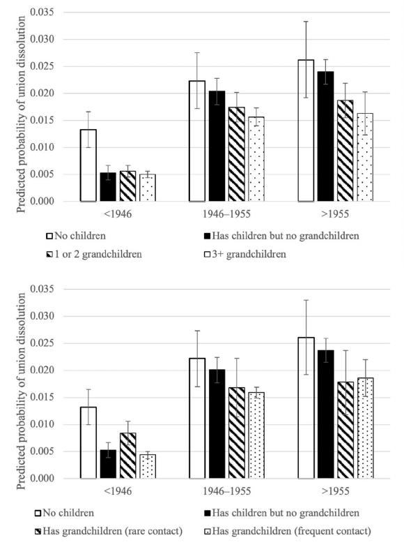
Panel A of Figure 2 shows the predicted probability with confidence intervals of late
union dissolution for childless individuals, those with children but no grandchildren,
those with one or two grandchildren, and those with three or more. Panel B shows the
predictions according to the variable about the intensity of family exchanges. First, both
figures clearly show that the probability of experiencing a silver split increases, on
average, among recent cohorts – especially among those born post-1955. Regarding
grandchildren (Panel A), the results suggest that the role of grandchildren in shaping
divorce behaviours has become increasingly important in younger generations. There is
a clear gradient among individuals born between 1946–1955 and those born after 1955,
suggesting that individuals with grandchildren are less prone to dissolve their unions after
the age of 50, especially if they have three or more grandchildren. For example, for those
born after 1955, the probability of late union dissolution for childless individuals was
approximately 2.6%; for individuals with children but no grandchildren it was 2.4%; and

Alderotti, Tomassini & Vignoli: ‘Silver splits’ in Europe: The role of grandchildren and other correlates
634 https://www.demographic-research.org
it was roughly 1.8% for those with one or two grandchildren and 1.6% for three or more
grandchildren. Such a gradient is slightly less evident in the 1946–1955 cohort, even if
the difference in the probability of silver splits between childless individuals and those
with more than two grandchildren is relatively large. These differences virtually
disappear in the oldest cohort (i.e., those born before 1946). In the oldest cohort, the
(predicted) probability of silver splits is much smaller than for the other cohorts and
remains virtually unchanged among the respondents with children, with one or two
grandchildren, and with three or more grandchildren. Panel B shows that the intensity of
family exchanges is a particularly relevant dimension for individuals from the older
cohorts. Indeed, the risk of silver splits is higher among individuals with grandchildren
who report having rare contact with their children (0.008), as compared to both
individuals with children but no grandchildren (0.005) and those who have grandchildren
and frequent contact with their children (0.004). Among the two younger cohorts, our
findings confirmed that having grandchildren is linked to a decrease in the probability of
experiencing late union dissolution (although the estimates have a low statistical
precision).
Table 2: Logistic model for the probability of experiencing union dissolution
after the age of 50. AMEs for the variables about children and
grandchildren are reported. N = 53,311
AME
p
-
value
Model 1
number of grandchildren (ref. childless)
has children, no grandchildren
–
0.0038
0.101
has one or two grandchildren
–
0.0065
0.006
has three or more grandchildren
–
0.0079
0.000
Model 2
contact with grandchildren (ref. childless)
has children, no grandchildren
–
0.0038
0.100
has children and grandchildren but rare contact
–
0.0057
0.065
has children and grandchildren with frequent contact
–
0.0077
0.000
Source: Authors’ elaboration on SHARE data, waves 1–7 (wave 3 excluded).
Note: The models control for gender, birth cohort, educational level, employment status, union duration, previous divorce experience,
homeownership, perceived financial stress, limitations with daily activities, depression scale, wave of entrance, and country of
residence.
Demographic Research: Volume 46, Article 21
https://www.demographic-research.org 635
Figure 2: Adjusted predicted probability of union dissolution by number of
grandchildren and birth cohort. Confidence intervals are reported
(A)
(B)
Source: Authors’ elaboration on SHARE data, waves 1–7 (wave 3 excluded).
Notes: Predicted probabilities are adjusted by gender, education level, employment status, union duration, previous divorce
experiences, homeownership, perceived financial stress, depression level, limitations in daily activities, and entrance wave. Predicted
probabilities refer to the population average.

Alderotti, Tomassini & Vignoli: ‘Silver splits’ in Europe: The role of grandchildren and other correlates
636 https://www.demographic-research.org
4.3 The other correlates of silver splits
Table 3 illustrates the relationship between the other variables and the risk of silver splits.
As expected, we found no difference by gender (AME = 0.0005, p-value = 0.505).
Individuals born between 1946–1955 and post-1955 (i.e., the baby boom cohorts) are
more likely to experience union dissolution than the oldest cohort (pre-1946). The model
highlighted no remarkable differences in the probability of silver splits according to
educational level (robust to different specifications of the education variable).
9
Regarding
employment status, retired individuals are more likely to experience a silver split than
those working or otherwise not retired. Our findings confirm that union duration is
negatively related to late union dissolution, meaning that the longer the marital duration,
the smaller the probability of experiencing a silver split. Previous divorce experiences
also play an important role in shaping silver split probability, with those who have already
divorced at least once being 9.95 pp more likely to experience a/another dissolution
compared to first-time divorcers. Homeownership is negatively related to silver split
probability, with a related AME of –0.0067 (p-value < 0.001). Regarding perceived
financial stress, we found that people who could make ends meet with difficulty or with
great difficulty had a higher probability of late union dissolution. Interestingly, regarding
health, we noted different results depending on the sphere of health considered. The
indicator for functional health revealed that a higher number of limitations in daily
activities related to a lower probability of late union dissolution (AME = –0.0020),
whereas we observed an opposing correlation for depression (AME = 0.0011). Finally,
those who entered the survey in the latest waves had a lower probability of late dissolution
(possibly due to their spending less time in observation).
9
We also tested education in the model as a binary variable with two different specifications: primary education
versus secondary or tertiary education, and primary or secondary education versus tertiary education.

Demographic Research: Volume 46, Article 21
https://www.demographic-research.org 637
Table 3: Logistic model for the probability of experiencing union dissolution
after the age of 50. AMEs are reported. N = 53,311
AME
p
-
value
gender (ref. male)
female
0.0005
0.505
birth
cohort (ref. before 1945)
1946
–
1955
0.0086
0.000
after
1955
0.0078
0.000
education (ref. primary)
secondary
–
0.0017
0.465
tertiary
0.0013
0.556
employment status (ref. retired)
working
–
0.0070
0.000
other (
e.g.,
unemployed, homemaker)
–
0.0093
0.000
union duration
–
0.0006
0.000
has already divorced at least once (ref. no)
yes
0.0995
0.000
homeowner
ship (ref. no)
yes
–
0.0067
0.000
making ends meet (ref. easily)
fairly easily
0.0024
0.214
with some difficulty
0.0041
0.017
with
great difficulty
0.0077
0.013
number of limitations with daily activities
–
0.0020
0.073
depression scale
0.0011
0.000
wave of entrance (ref. wave 1)
wave 2
0.0006
0.861
wave 4
–
0.0029
0.049
wave 5
–
0.0062
0.004
wave 6
–
0.0125
0.000
number of
grandchildren
YES
c
ountry fixed effects
YES
Source: Authors’ elaboration on SHARE data, waves 1–7 (wave 3 excluded).
4.4 Robustness checks and further analyses
Our findings are confirmed across various additional analyses and robustness checks.
Due to space constraints, the results are not shown here but are available upon request.
First, we added an interaction term between the number of children and the country of
residence in order to consider possible country-level differences but found no relevant
result (quite possibly due to reduced sample size). Moreover, to operationalise the ‘empty
nest’ concept, we also tested interaction terms between the number of grandchildren and
the fact that none, some, or all children had left the parental home. However, the cells
Alderotti, Tomassini & Vignoli: ‘Silver splits’ in Europe: The role of grandchildren and other correlates
638 https://www.demographic-research.org
became too small and yielded inconclusive results. Regarding the role of children, we
conducted a specific analysis to check whether the number of children was also
significant and found that individuals with two or more children are less likely to
experience silver splits than those with only one child. Additionally, since we used
multiple imputation techniques to manage missing information, all models estimated on
the imputed dataset were replicated on the original dataset (i.e., without imputations).
While the estimates remained virtually unchanged, they clearly lost part of their statistical
precision. Finally, we replicated the analysis excluding individuals whose missing
information was recovered from previous waves. Again, the results remain virtually
unchanged but lost part of their statistical precision due to the reduced sample size.
5. Conclusions
Union dissolution in later life has become increasingly relevant as a social and
demographic phenomenon. Despite this growing importance, the correlates of silver
splits remain underexplored – especially in Europe. Using data from six waves of the
SHARE dataset, we explored the role of several factors as potential correlates of late
union dissolution, with a special emphasis on the role of children and grandchildren. We
studied union dissolution rather than divorce in the strict sense of the word to
acknowledge the increasing diversity of family life at older ages.
Our analysis suggests that having children and grandchildren is associated with a
lower probability of experiencing a silver split. Indeed, we found that late union
dissolution is less likely when individuals have children, let alone grandchildren. This
finding is unsurprising and aligns with prior research showing that having children is a
well-established factor that consolidates unions among the analysed birth cohorts (e.g.,
De Rose 1992; Hoem and Hoem 1992; Lyngstad and Jalovaara 2010; White 1990), and
that family-oriented individuals are both more likely to have children and less likely to
dissolve their union (Lesthaeghe and Moors 2000). Becker, Landes, and Michae (1977)
observe that children are a ‘marital-specific capital,’ thus representing a sign of family
harmony with positive implications for union stability. However, it remains to be seen
whether this association will be confirmed in future generations.
The effect of grandchildren in shaping silver splits is especially interesting. To
explore this effect, we employed two variables (the number of grandchildren and the
intensity of family exchanges) and explored their relationship with the risk of a silver
split. Our findings indicate that having grandchildren reduces this risk and that both their
number and the frequency of contact with children and grandchildren play a significant
role. Not only having grandchildren but also maintaining frequent contact with them
relates to a lower probability of late union dissolution. While it has been widely
Demographic Research: Volume 46, Article 21
https://www.demographic-research.org 639
established that having children is a strong inhibitor to divorce at younger ages (i.e., when
children are young), as children (and parents) age, this relationship may weaken. At later
ages, having grandchildren – in addition to that of children – and the intensity of family
exchanges influence the probability of union dissolution, possibly due to the positive
relationship between becoming grandparents and individual well-being (e.g., Arpino,
Bordone, and Balbo 2018). Interestingly, this correlation differs across birth cohorts. On
the one hand, younger cohorts have higher divorce rates than their older counterparts, and
childless individuals are always the most likely to experience late union dissolutions. On
the other hand, our findings suggest that, compared to individuals who only have
children, those who have also grandchildren have an even lower risk of silver splits –
especially among those born after 1946. This result may be explained by the fact that
more recent cohorts have young grandchildren whose grandparents are more involved in
childcare (which may be a form of positive engagement for the couple) compared to those
with older grandchildren who are less in need of care (Pasqualini, Di Gessa, and
Tomassini 2021). However, such an interpretation should be made cautiously since the
timing of fertility and childcare attitudes have changed over time and differ between
countries.
As an ancillary but important outcome of the study, we suggest that the European
correlates of silver splits are similar to those found previously in a North American
context. Regarding birth cohorts, we found that individuals born after 1946 were more
likely to experience late union dissolutions than those born previously. This aligns with
previous findings in the United States showing that the baby boom cohorts are the most
prone to divorce and sparked the silver split phenomenon as they aged (Brown and Lin
2012; Cohen 2019; Lin et al. 2018). We confirmed union duration to be negatively related
to silver splits, while previous divorce experiences proved to be important predictors of
silver splits at later ages. Retired individuals have a higher risk of experiencing union
dissolution after the age of 50 compared to those not retired. Regarding economic
conditions, our findings suggest a positive correlation between financial stress and silver
splits since individuals who struggle to make ends meet are more likely to dissolve their
unions after the age of 50, and homeowners are less likely to experience a silver split
compared to those who do not own a house. The latter finding suggests that a stable
housing situation may improve marital quality in later life, which accords with previous
research on the importance of housing for the aged (Angelini, Laferrère, and Weber 2013;
Vignoli, Tanturri, and Acciai 2016). Finally, our study supports the hypothesis of a
negative relationship between deteriorating mental health (i.e., depression) and late union
dissolution, thereby corroborating previous findings (Davies, Avison, and McAlpine
1997; Idstad et al. 2015; Kessler, Walters, and Forthofer 1998; Torvik et al. 2015).
Conversely, we found that poor physical health – measured through the number of
limitations to daily activities – was associated with a reduced likelihood of union
Alderotti, Tomassini & Vignoli: ‘Silver splits’ in Europe: The role of grandchildren and other correlates
640 https://www.demographic-research.org
dissolution. Education level seemed irrelevant to silver splits. This is in line with existing
studies showing that educational level has only a limited effect on the probability of grey
divorce in the United States (Brown and Lin 2012; Lin et al. 2018).
It would be important to note several limitations to our study. First, the small number
of cases prohibited a country-specific analysis. This means that our findings reveal
average effects computed across several countries and thus obscure any potential
country-specific patterns. Furthermore, it is possible that we found no association
between some factors (e.g., education) and silver splits simply because opposing country-
specific effects averaged out. Another limitation relates to attrition. Different solutions
have been proposed on how to most effectively control for attrition, depending on the
mechanisms generating loss at follow-up (see e.g., Enders 2010; Little and Rubin 2002).
Although attrition effects are present in most panel surveys to various extents, their
consequences on model results are often disregarded in demographic research, which
may lead to a non-negligible bias (Alderman et al. 2001). Despite our efforts to include
a wide array of control variables in the models in order to mitigate attrition bias, such a
solution can reduce the consequences of attrition only to the extent that it depends on
observable characteristics. Nevertheless, it is worth noting that previous analyses have
found little evidence of selective attrition bias in SHARE (Bergmann et al. 2017; Kneip,
Malter, and Sand 2015). We also encountered certain data limitations. We were unable
to follow a couple approach because a substantial number of participants had (totally or
partially) nonresponding partners, who would have introduced a further selection in our
analyses. Besides, due to the reduced number of cases, we made no distinctions between
biological children and step-children, nor did we do so for biological grandchildren and
step-grandchildren. We found inconsistencies in marital and partner status across waves
(e.g., individuals who were married in one wave and reported being single in the
following one). Furthermore, approximately 5,000 individuals reported missing
information about their union duration, upon which we opted to impute these missing
values. Finally, we inferred family intensity through information concerning the
frequency of contact with children, which may possibly have introduced a bias.
Unfortunately, information about the frequency of contact with grandchildren was not
available, and data regarding whether the respondent cares for grandchildren were
accessible only if the latter was younger than 13 years of age.
Despite these limitations, this paper sheds some light on the correlates of a rare but
demographically and sociologically relevant phenomenon. Having children has been
widely shown to inhibit union dissolution – especially among older cohorts. Indeed,
parents may postpone their marital dissolution until after the ‘empty nest’ phase for the
sake of their children. However, grandchildren may serve to ‘refill the nest,’ thus
discouraging silver splits as grandparents assume new familial and social responsibilities.
Although predominantly exploratory, our study expands existing knowledge on the
Demographic Research: Volume 46, Article 21
https://www.demographic-research.org 641
factors related to silver splits in Europe and, we hope, will feed future research on the
topic (e.g., scrutinising the role of children and grandchildren specifically by country and
gender, or investigating potential differences between biological grandchildren and step-
grandchildren).
6. Acknowledgements
This paper uses data from SHARE Waves 1, 2, 4, 5, 6, and 7 (DOIs: 10.6103/
SHARE.w1.800, 10.6103/SHARE.w2.800, 10.6103/SHARE.w4.800, 10.6103/SHARE.
w5.800, 10.6103/SHARE.w6.800, 10.6103/SHARE.w7.800), see Börsch-Supan et al.
(2013) for methodological details. The SHARE data collection has been funded by the
European Commission, DG RTD through FP5 (QLK6-CT-2001-00360), FP6 (SHARE-
I3: RII-CT-2006-062193, COMPARE: CIT5-CT-2005-028857, SHARELIFE: CIT4-
CT-2006-028812), FP7 (SHARE-PREP: GA N°211909, SHARE-LEAP: GA N°227822,
SHARE M4: GA N°261982, DASISH: GA N°283646) and Horizon 2020 (SHARE-
DEV3: GA N°676536, SHARE-COHESION: GA N°870628, SERISS: GA N°654221,
SSHOC: GA N°823782, SHARE-COVID19: GA N°101015924) and by DG
Employment, Social Affairs & Inclusion through VS 2015/0195, VS 2016/0135, VS
2018/0285, VS 2019/0332, and VS 2020/0313. Additional funding from the German
Ministry of Education and Research, the Max Planck Society for the Advancement of
Science, the U.S. National Institute on Aging (U01_AG09740-13S2, P01_AG005842,
P01_AG08291, P30_AG12815, R21_AG025169, Y1-AG-4553-01, IAG_BSR06-11,
OGHA_04-064, HHSN271201300071C, RAG052527A) and from various national
funding sources is gratefully acknowledged (see www.share-project.org).
The authors acknowledge the financial support provided by the Italian Ministry of
University and Research under the 2017 MiUR-PRIN Grant Prot. N. 2017W5B55Y
(“The Great Demographic Recession,” PI: Daniele Vignoli). The authors would also like
to thank the project “Care, Retirement and Wellbeing of Older People Across Different
Welfare Regimes” (CREW), and the colleagues from the Unit of Population and Society
(UPS) of the University of Florence for their much-valued comments.
Alderotti, Tomassini & Vignoli: ‘Silver splits’ in Europe: The role of grandchildren and other correlates
642 https://www.demographic-research.org
References
Aassve, A., Arpino, B., and Billari, F.C. (2013). Age norms on leaving home: Multilevel
evidence from the European Social Survey. Environment and Planning A 45(2):
383–401. doi:10.1068/a4563.
Alcser, K.H., Benson, G., Börsch-Supan, A., Brugiavini, A., Christelis, D., Croda, E.,
and Weerman, B. (2005). The survey of health, aging, and retirement in Europe –
Methodology. Mannheim Mannheim Research Institute for the Economics of
Aging.
Alderman, H., Behrman, J.R., Kohler, H.-P., Maluccio, J.A., and Watkins, S.C. (2001).
Attrition in longitudinal household survey data: Some tests for three developing-
country samples. Demographic Research 5(4): 79–124. doi:10.4054/DemRes.
2001.5.4.
Amato, P.R. (2010). Research on divorce: Continuing trends and new developments.
Journal of Marriage and the Family 72(3): 650–666. doi:10.1111/j.1741-
3737.2010.00723.x.
Angelini, V., Laferrère, A., and Weber, G. (2013). Home-ownership in Europe: How did
it happen? Advances in Life Course Research 18(1): 83–90. doi:10.1016/j.alcr.
2012.10.006.
Arpino, B., Bordone, V., and Balbo, N. (2018). Grandparenting, education and subjective
well-being of older Europeans. European Journal of Ageing 15(3): 251–263.
doi:10.1007/s10433-018-0467-2.
Bair, D. (2007). Calling it quits: Late life divorce and starting over. New York, NY:
Random House
Becker, G.S., Landes, E.M., and Michael, R.T. (1977). An economic analysis of marital
instability. Journal of Political Economy 85(6): 1141–1188. doi:10.1086/260631.
Berger, P. and Kellner, H. (1964). Marriage and the construction of reality: An exercise
in the microsociology of knowledge. Diogenes 12(46): 1–24. doi:10.1177/0392
19216401204601.
Bergmann, M., Kneip, T., De Luca, G., and Scherpenzeel, A. (2017). Survey participation
in the survey of health, ageing and retirement in Europe (SHARE), Wave 1–6.
Munich: Munich Center for the Economics of Aging.
Demographic Research: Volume 46, Article 21
https://www.demographic-research.org 643
Bernardi, L., Huinink, J., and Settersten Jr, R.A. (2019). The life course cube: A tool for
studying lives. Advances in Life Course Research 41: 100258. doi:10.1016/j.alcr.
2018.11.004.
Blossfeld, H.-P., de Rose, A., Hoem, J.M., and Rohwer, G. (1995). Education,
modernization, and the risk of marriage disruption in Sweden, West Germany, and
Italy. In: Oppenheim Mason, K. and Jensen, A.-M. (eds.). Gender and family
change in industrialized countries. Oxford: Clarendon Press: 200–222.
Börsch-Supan, A., Brandt, M., Hunkler, C., Kneip, T., Korbmacher, J., Malter, F.,
Schaan, B., Stuck, S., and Zuber, S. (2013). Data resource profile: The Survey of
Health, Ageing and Retirement in Europe (SHARE). International Journal of
Epidemiology 42(4): 992–1001. doi:10.1093/ije/dyt088.
Booth, A. and Johnson, D. R. (1994). Declining health and marital quality. Journal of
Marriage and the Family 56(1): 218–223. doi:10.2307/352716.
Brines, J. and Joyner, K. (1999). The ties that bind: Principles of cohesion in cohabitation
and marriage. American Sociological Review 64(3): 333–355. doi:10.2307/2657
490.
Brown, S.L. and Lin, I.F. (2012). The gray divorce revolution: Rising divorce among
middle-aged and older adults, 1990–2010. The Journals of Gerontology Series B:
Psychological Sciences and Social Sciences 67(6): 731–741. doi:10.1093/geronb/
gbs089.
Brown, S.L. and Wright, M.R. (2019). Divorce attitudes among older adults: Two
decades of change. Journal of Family Issues 40(8): 1018–1037. doi:10.1177/
0192513X19832936.
Brown, S.L., Lin, I.F., and Mellencamp, K.A. (2021). Does the transition to
grandparenthood deter gray divorce? A test of the braking hypothesis. Social
Forces 99(3): 1209–1232. doi:10.1093/sf/soaa030.
Bukodi, E. and Robert, P. (2003). Union disruption in Hungary. International Journal of
Sociology 33(1): 64–94. doi:10.1080/15579336.2003.11770264.
Canham, S.L., Mahmood, A., Stott, S., Sixsmith, J., and O’Rourke, N. (2014). ‘Til
divorce do us part: Marriage dissolution in later life. Journal of Divorce and
Remarriage 55(8): 591–612. doi:10.1080/10502556.2014.959097.
Chan, T.W. and Halpin, B. (2002). Union dissolution in the United Kingdom.
International Journal of Sociology 32(4): 76–93. doi:10.1080/15579336.2002.11
770260.
Alderotti, Tomassini & Vignoli: ‘Silver splits’ in Europe: The role of grandchildren and other correlates
644 https://www.demographic-research.org
Charles, K.K. and Stephens, Jr, M. (2004). Job displacement, disability, and divorce.
Journal of Labor Economics 22(2): 489–522. doi:10.1086/381258.
Cohen, P.N. (2019). The coming divorce decline. Socius 5. doi:10.1177/237802311
9873497.
Crowley, J.E. (2019). Does everything fall apart? Life assessments following a gray
divorce. Journal of Family Issues 40(11): 1438–1461. doi:10.1177/0192513X1
9839735.
Cunningham-Burley, S. (1986). Becoming a grandparent. Ageing and Society 6(4): 453–
470. doi:10.1017/S0144686X00006267.
Daniel, K., Wolfe, C.D., Busch, M.A., and McKevitt, C. (2009). What are the social
consequences of stroke for working-aged adults? A systematic review. Stroke
40(6): e431–e440. doi:10.1161/STROKEAHA.108.534487.
Davies, L., Avison, W.R., and McAlpine, D.D. (1997). Significant life experiences and
depression among single and married mothers. Journal of Marriage and the
Family 59(2): 294–308. doi:10.2307/353471.
De Jong Gierveld, J., van Tilburg, T.G., and Dykstra, P.A. (2016). Loneliness and social
isolation. In: Vangelisti, A. and Perlman, D. (eds.). The Cambridge handbook of
personal relationships. Cambridge, MA: Cambridge University Press: 485–500.
doi:10.1017/CBO9780511606632.027.
De Rose, A. (1992). Socio-economic factors and family size as determinants of marital
dissolution in Italy. European Sociological Review 8(1): 71–91. doi:10.1093/
oxfordjournals.esr.a036623.
De Shane, M.R. and Brown-Wilson, K. (1982). Divorce in late life: A call for research.
Journal of Divorce 4(4): 81–91. doi:10.1300/J279v04n04_06.
Drew, L.M. and Silverstein, M. (2007). Grandparents’ psychological well-being after loss
of contact with their grandchildren. Journal of Family Psychology 21(3): 372.
doi:10.1037/0893-3200.21.3.372.
Drew, L.M. and Smith, P.K. (2002). Implications for grandparents when they lose contact
with their grandchildren: Divorce, family feud and geographical separation.
Journal of Mental Health and Aging 8: 95–120.
Elder Jr, G.H. (1994). Time, human agency, and social change: Perspectives on the life
course. Social Psychology Quarterly 57(1): 4–15. doi:10.2307/2786971.
Enders, C.K. (2010). Applied missing data analysis. Guilford Press.
Demographic Research: Volume 46, Article 21
https://www.demographic-research.org 645
Esterberg, K.G., Moen, P., and Dempster‐McCain, D. (1994). Transition to divorce: A
life‐course approach to women’s marital duration and dissolution. Sociological
Quarterly 35(2): 289–307. doi:10.1111/j.1533-8525.1994.tb00411.x.
Gaymu, J. (2003). The housing conditions of elderly people. Genus 59(1): 201–226.
Glenn, N.D. and Supancic, M. (1984) The social and demographic correlates of divorce
and separation in the United States: An update and reconsideration. Journal of
Marriage and Family 46(3): 563–575. doi:10.2307/352598.
Goldstein, H. and Healy, M.J. (1995). The graphical presentation of a collection of
means. Journal of the Royal Statistical Society: Series A (Statistics in Society)
158(1): 175–177. doi:10.2307/2983411.
Hank, K., Cavrini, G., Di Gessa, G., and Tomassini, C. (2018). What do we know about
grandparents? Insights from current quantitative data and identification of future
data needs. European Journal of Ageing 15(3): 225–235. doi:10.1007/s10433-
018-0468-1.
Hiedemann, B., Suhomlinova, O., and O’Rand, A.M. (1998). Economic independence,
economic status, and empty nest in midlife marital disruption. Journal of
Marriage and Family 60(1): 219–231. doi:10.2307/353453.
Hoem, B. and Hoem, J.M. (1992). Disruption of marital and non-marital unions in
Sweden. In: Trussell, J., Hankinson, R., and Tilton, J. (eds.). Demographic
applications of event history analysis. Oxford: Clarendon Press.
Hoem, J.M. (1997). Educational gradients in divorce risks in Sweden in recent decades.
Population Studies 51(1): 19–27. doi:10.1080/0032472031000149696.
Hoem, J.M. and Kreyenfeld, M. (2006). Anticipatory analysis and its alternatives in life-
course research. Part 1: The role of education in the study of first
childbearing. Demographic Research 15(16): 461–484. doi:10.4054/DemRes.
2006.15.16.
Idstad, M., Torvik, F.A., Borren, I., Rognmo, K., Røysamb, E., and Tambs, K. (2015).
Mental distress predicts divorce over 16 years: the HUNT study. BMC Public
Health 15(320). doi:10.1186/s12889-015-1662-0.
Jalovaara, M. (2001). Socio-economic status and divorce in first marriages in Finland
1991–93. Population Studies 55(2): 119–133. doi:10.1080/00324720127685.
Jalovaara, M. (2002). Socioeconomic differentials in divorce risk by duration of
marriage. Demographic Research 7(16): 537–564. doi:10.4054/DemRes.2002.
7.16.

Alderotti, Tomassini & Vignoli: ‘Silver splits’ in Europe: The role of grandchildren and other correlates
646 https://www.demographic-research.org
Joung, I.M., Van De Mheen, H.D., Stronks, K., Van Poppel, F.W., and Mackenbach, J.P.
(1998). A longitudinal study of health selection in marital transitions. Social
Science and Medicine 46(3): 425–435. doi:10.1016/S0277-9536(97)00186-X.
Karraker, A. and Latham, K. (2015) In sickness and in health? Physical illness as a risk
factor for marital dissolution in later life. Journal of Health and Social Behavior
56(3): 420–435. doi:10.1177/0022146515596354.
Kennedy, S. and Ruggles, S. (2014). Breaking up is hard to count: The rise of divorce in
the United States, 1980–2010. Demography 51(2): 587–598. doi:10.1007/s13524-
013-0270-9.
Kessler, R.C., Walters, E.E., and Forthofer, M.S. (1998) The social consequences of
psychiatric disorders, III: Probability of marital stability. American Journal of
Psychiatry 155(8): 1092–1096. doi:10.1176/ajp.155.8.1092.
King, V. (2003), The legacy of a grandparent’s divorce: Consequences for ties between
grandparents and grandchildren. Journal of Marriage and Family 65(1): 170–183.
doi:10.1111/j.1741-3737.2003.00170.x.
Kneip, T., Malter, F., and Sand, G. (2015). Fieldwork monitoring and survey
participation in fifth wave of SHARE. SHARE wave 5: 102–159.
Kulu, H. and Boyle, P.J. (2010). Premarital cohabitation and divorce: Support for the
“Trial Marriage” Theory? Demographic Research 23(31): 879–904. doi:10.4054/
DemRes.2010.23.31.
Kulu, H. (2014). Marriage duration and divorce: The seven-year itch or a lifelong itch?
Demography 51(3): 881–893. doi:10.1007/s13524-013-0278-1.
Lee, K.J. and Carlin, J.B. (2010). Multiple imputation for missing data: Fully conditional
specification versus multivariate normal imputation. American Journal of
Epidemiology 171(5): 624–632. doi:10.1093/aje/kwp425.
Lesthaeghe, R. and Moors, G.B.D. (2000). Recent trends in fertility and household
formation in the industrialised world. Review of Population and Social Policy 9:
121–170.
Lin, I.F., Brown, S., Wright, M., and Hammersmith, A. (2018) Antecedents of gray
divorce: A life course perspective. The Journals of Gerontology Series B:
Psychological Sciences and Social Sciences 73(6): 1022–1031.
Little, R.J. and Rubin, D.B. (2002). Bayes and multiple imputation. In: Statistical
analysis with missing data. Hoboken: John Wiley and Sons, Inc.: 200–220.
doi:10.1002/9781119013563.ch10.
Demographic Research: Volume 46, Article 21
https://www.demographic-research.org 647
Lyngstad, T.H. and Jalovaara, M. (2010) A review of antecendents of union dissolution
Demographic Research 23(10): 257–292. doi:10.4054/DemRes.2010.23.10.
Martin, S.P. (2006). Trends in marital dissolution by women’s education in the United
States. Demographic Research 15(20): 537–560. doi:10.4054/DemRes.2006.
15.20.
Mastekaasa, A. (1994). Psychological well-being and marital dissolution – Selection
effects. Journal of Family Issues 15(2): 208–228. doi:10.1177/0192513X940
15002004.
Matysiak, A., Styrc, M., and Vignoli, D. (2014). The educational gradient in marital
disruption: A meta-analysis of European research findings. Population Studies
68(2): 197–215. doi:10.1080/00324728.2013.856459.
Office for National Statistics (2017). Marriage and divorce on the rise at 65 and over.
https://www.ons.gov.uk/peoplepopulationandcommunity/birthsdeathsandmarriag
es/marriagecohabitationandcivilpartnerships/articles/marriageanddivorceontheris
eat65andover/2017-07-18.
Ono, H. (1999). Historical time and US marital dissolution. Social Forces 77(3): 969–
999. doi:10.2307/3005968.
Pasqualini, M., Di Gessa, G., and Tomassini, C. (2021). A change is (not) gonna come:
a 20-year overview of Italian grandparent–grandchild exchanges. Genus 77(1): 1–
25. doi:10.1186/s41118-021-00142-6.
Pezzin, L.E. and Schone, B.S. (1999). Parental marital disruption and intergenerational
transfers: an analysis of lone elderly parents and their children. Demography
36(3): 287–297. doi:10.2307/2648053.
Poortman, A.R. and Kalmijn, M. (2002). Women’s labour market position and divorce
in the Netherlands: Evaluating economic interpretations of the work effect.
European Journal of Population/Revue europeenne de demographie 18(2): 175–
202. doi:10.1023/A:1015520411449.
Prince, M.J., Beekman, A.T., Deeg, D.J., Fuhrer, R., Kivela, S.L., Lawlor, B.A., and
Reischies, F. (1999). Depression symptoms in late life assessed using the EURO–
D scale. The British Journal of Psychiatry 174(4): 339–345. doi:10.1192/bjp.
174.4.339.
Raley, R.K. and Sweeney, M.M. (2020). Divorce, repartnering, and stepfamilies: A
decade in review. Journal of Marriage and Family 82(1): 81–99. doi:10.1111/
jomf.12651.
Alderotti, Tomassini & Vignoli: ‘Silver splits’ in Europe: The role of grandchildren and other correlates
648 https://www.demographic-research.org
Rotz, D. (2016). Why have divorce rates fallen? The role of women’s age at marriage.
Journal of Human Resources 51(4): 961–1002. doi:10.3368/jhr.51.4.0214-6224R.
Rubin, D.B. (1987). Multiple imputation for nonresponse in surveys. New York: Wiley.
doi:10.1002/9780470316696.
Solaz, A. (2021). More frequent separation and repartnering among people aged 50 and
over. Population Societies (2): 1–4.
Svarer, M. and Verner, M. (2006). Do children stabilize Danish marriages? Journal of
Population Economics 21(2): 395–417. doi:10.1007/s00148-006-0084-9.
Tomassini, C., Kalogirou, S., Grundy, E., Fokkema, T., Martikainen, P., Van Groenou,
M.B., and Karisto, A. (2004). Contacts between elderly parents and their children
in four European countries: current patterns and future prospects. European
Journal of Ageing 1(1): 54–63. doi:10.1007/s10433-004-0003-4.
Torvik, F.A., Gustavson, K., Røysamb, E., and Tambs, K. (2015) Health, health
behaviors, and health dissimilarities predict divorce: results from the HUNT
study. BMC Psychology 3(13). doi:10.1186/s40359-015-0072-5.
Tosi, M. and Van den Broek, T. (2020). Gray divorce and mental health in the United
Kingdom. Social Science and Medicine 256: 113030. doi:10.1016/j.socscimed.
2020.113030.
Uhlenberg, P., Cooney, T., and Boyd, R. (1990). Divorce for women after midlife.
Journal of Gerontology: Social Sciences 45(1): S3–11. doi:10.1093/geronj/45.
1.S3.
Uhlenberg, P. and Hammill, B.G. (1998). Frequency of grandparent contact with
grandchild sets: Six factors that make a difference. The Gerontologist 38(3): 276–
285. doi:10.1093/geront/38.3.276.
Vignoli, D. and Ferro, I. (2009). Rising marital disruption in Italy and its correlates.
Demographic Research 20(4): 11–36. doi:10.4054/DemRes.2009.20.4.
Vignoli, D., Matysiak, A., Styrc, M., and Tocchioni, V. (2018). The positive impact of
women’s employment on divorce: Context, selection, or anticipation?
Demographic Research 38(37): 1059–1110. doi:10.4054/DemRes.2018.38.37.
Vignoli, D., Tanturri, M.L., and Acciai, F. (2016). Home bitter home? Gender, living
arrangements, and the exclusion from homeownership among older Europeans.
Genus 72(1): 9. doi:10.1186/s41118-016-0014-y.
Demographic Research: Volume 46, Article 21
https://www.demographic-research.org 649
Weingarten, H.R. (1988). Late life divorce and the life review. Journal of Gerontological
Social Work 12(3–4): 83–97. doi:10.1300/J083v12n03_06.
White, L.K. (1990). Determinants of divorce: A review of research in the eighties.
Journal of Marriage and the Family 52(4): 904–912. doi:10.2307/353309.
Wilson, S.E. and Waddoups, S.L. (2002). Good marriages gone bad: Health mismatches
as a cause of later-life marital dissolution. Population Research and Policy Review
21(6): 505–533. doi:10.1023/A:1022990517611.
Wu, Z. and Penning, M.J. (1997). Marital instability after midlife. Journal of Family
Issues 18(5): 459–478. doi:10.1177/019251397018005001.
Wu, Z. and Penning, M.J. (2018). Marital and cohabiting union dissolution in middle and
later life. Research on Aging 40(4): 340–364. doi:10.1177/0164027517698024.
Yorgason, J.B., Booth, A., and Johnson, D. (2008). Health, disability, and marital quality:
Is the association different for younger versus older cohorts? Research on Aging
30(6): 623–648. doi:10.1177/0164027508322570.
Alderotti, Tomassini & Vignoli: ‘Silver splits’ in Europe: The role of grandchildren and other correlates
650 https://www.demographic-research.org
Appendix
Sample attrition
We investigated the factors associated with the probability of not entering our analytical
sample (i.e., participating in the survey only once). Table A-1 shows the results of a
logistic regression for the probability of leaving the survey after only one interview. We
reported four-digit AMEs in order to avoid rough approximations due to the small
magnitude of coefficients. Respondents who died after their first participation were
excluded from the model (n = 1,802, or approximately 10% of those who left). The model
revealed no relevant gender difference, while people born after 1955 were more likely to
abandon the survey after one wave (it should be noted that we did not consider leaving
the survey due to death as attrition). The probability of attrition was 2.67% lower among
people with tertiary education. Regarding employment status, retired individuals were
the least likely to leave the survey, while the employed and otherwise unretired had a
higher attrition risk. Having children was negatively related to attrition: Individuals with
one child and those with two or more were 2% and 6.6% less likely to leave the sample,
respectively. Having already had previous divorce experiences did not relevantly affect
the probability of attrition. Homeownership was related to a lower probability of attrition,
and those who reported finding it easy to make ends meet were the least likely to leave
due to attrition. These last two findings suggest that individuals with higher
socioeconomic status may be less inclined to terminate their participation. Finally,
limitations in daily activities played no prominent role, while depression was associated
with lower attrition probability (AME = –0.003). All the factors considered in Table 1
were included in the models on the probability of union dissolution due to their
correlation with attrition probabilities.

Demographic Research: Volume 46, Article 21
https://www.demographic-research.org 651
Table A-1: Logistic model for the probability of leaving the survey after one
wave. AMEs are reported. N = 72,032
AME
p
-
value
gender (ref. male)
female
–
0.0022
0.631
birth cohort (ref. before 1945)
1946
–
1955
–
0.0071
0.507
after 1955
0.0274
0.098
education (ref. primary)
secondary
–
0.0108
0.202
T
ertiary
–
0.0267
0.000
employment status (ref. retired)
working
0.0221
0.012
other (
e.g.,
unemployed, homemaker)
0.0141
0.059
number of children (ref. childless)
one child
–
0.0201
0.062
two or more children
–
0.0659
0.000
has already divorced at least once (ref. no)
yes
–
0.0054
0.538
homeowner
ship (ref. no)
yes
–
0.0294
0.000
making ends meet (ref. easily)
fairly easily
0.0139
0.050
with some difficulty
0.0135
0.222
with great difficulty
0.0001
0.934
number of limitations with daily activities
0.0042
0.210
depression scale
–
0.0030
0.043
c
ountry fixed effects
YES
w
ave
YES
Source: Authors’ elaboration on SHARE data, waves 1–7 (wave 3 excluded).

Alderotti, Tomassini & Vignoli: ‘Silver splits’ in Europe: The role of grandchildren and other correlates
652 https://www.demographic-research.org
Figure A-1: Flow chart of the sample selection process
72,032 eligible observations
(i.e., they were (1) married or in a registered cohabitation or (2) in an
informal relationship involving cohabitation at the time of the interview)
18,721 observations lost at follow up (i.e.,
they were interviewed only once)
Analytical sample:
53,311 observations interviewed at least twice
Out of the 53,311
observations:
17,392 left the survey
before the last wave
(potential attrition)
3,448 left because of
death
135 left after
experiencing union
13,809 left because of
attrition
1,831 out of 13,809: information
recovered through the partner
135 left after experiencing
union dissolution
