
1/33
Fast Bayesian A/B and multivariate testing
Guillermo Navas Palencia
BBVA, Global Risk Management – Analytics
PyDay BCN 2019
Barcelona, 16
th
November 2019


3/33
Introduction (1 / 2)
I
Frequentist inference (classical inference / classical point estimation)
I
Base on asymptotic performance =⇒ Central Limit Theorem (CLT).
I
P-value: the probability of seeing a result at least as extreme as a real result
after a A/A test of the same size [Stu15]. It is defined as
p-value = P[t ≥ t
e
|H
0
], H
0
: B ≡ A
I
Hypothesis testing based on rejecting H
0
. p-value 6= P[B > A]!
I
Confidence interval: if we repeated the same experiment used to construct
an interval for an unobserved value n times (n → ∞), (100 − δ)% of the
intervals would contain the true value. This is not a credible interval!
I
Set and fix stopping rule and sample size (power test calculation).
I
Bayesian inference
I
Bayes Theorem: given a prior distribution p(θ), update belief based on
sample x
p(θ|x) =
f (x|θ)p(θ)
f (x)
I
Choose of prior parameters =⇒ update =⇒ posterior parameters.
I
Calculation of posterior distribution.
I
Calculation of predictive posterior distribution.

4/33
Introduction (2 / 2)
I
Bayesian inference: advantages
I
Ease interpretability.
I
Sample size is not fixed in advance =⇒ repeated/streaming testing.
I
Account for uncertainty; points estimates =⇒ random variables.
I
Immune to data peeking
I
Bayesian inference: disadvantages
I
Analytical tractability
I
Computational cost

5/33
Bayesian testing metrics: probability to beat
I
A/B testing: the error probability or probability of X
B
> X
A
E (B) = P[X
B
> X
A
]
>>> from scipy import stats
>>> xa = stats.beta(2, 10).rvs(size=int(1e6))
>>> xb = stats.beta(3, 12).rvs(size=int(1e6))
>>> (xb > xa).mean()
I
Multivariate testing: the probability to beat all
E (X
i
) = P
X
i
> max
j6=i
X
j
>>> import numpy as np
>>> from scipy import stats
>>> xa = stats.beta(2, 10).rvs(size=int(1e6))
>>> xb = stats.beta(3, 12).rvs(size=int(1e6))
>>> xc = stats.beta(5, 60).rvs(size=int(1e6))
>>> xd = stats.beta(7, 90).rvs(size=int(1e6))
>>> maxall = np.maximum.reduce([xa, xc, xd])
>>> (xb > maxall).mean()

6/33
Bayesian testing metrics: expected loss
I
A/B testing: the expected value of the loss function
EL(B) = E[max(X
A
− X
B
, 0)]
>>> import numpy as np
>>> from scipy import stats
>>> xa = stats.beta(2, 10).rvs(size=int(1e6))
>>> xb = stats.beta(3, 12).rvs(size=int(1e6))
>>> np.maximum(xa - xb, 0).mean()
I
Multivariate testing: the expected loss function vs all
EL(X
i
) = E[ max(max
j6=i
X
j
− X
i
, 0)]
>>> import numpy as np
>>> from scipy import stats
>>> xa = stats.beta(2, 10).rvs(size=int(1e6))
>>> xb = stats.beta(3, 12).rvs(size=int(1e6))
>>> xc = stats.beta(5, 60).rvs(size=int(1e6))
>>> xd = stats.beta(7, 90).rvs(size=int(1e6))
>>> maxall = np.maximum.reduce([xa, xc, xd])
>>> np.maximum(maxall - xb, 0).mean()

7/33
Bayesian testing metrics: expected relative loss
I
A/B testing: the expected value of the relative loss function
ERL(B) = E[(X
A
− X
B
)/X
B
]
>>> import numpy as np
>>> from scipy import stats
>>> xa = stats.beta(2, 10).rvs(size=int(1e6))
>>> xb = stats.beta(3, 12).rvs(size=int(1e6))
>>>((xa - xb) / xb).mean()
I
Multivariate testing: the expected relative loss function vs all
ERL(X
i
) = E[ (max
j6=i
X
j
− X
i
)/X
i
]
>>> import numpy as np
>>> from scipy import stats
>>> xa = stats.beta(2, 10).rvs(size=int(1e6))
>>> xb = stats.beta(3, 12).rvs(size=int(1e6))
>>> xc = stats.beta(5, 60).rvs(size=int(1e6))
>>> xd = stats.beta(7, 90).rvs(size=int(1e6))
>>> maxall = np.maximum.reduce([xa, xc, xd])
>>> ((maxall - xb) / xb).mean()

8/33
Computation of credible intervals
Definition: A credible interval is a region with a particular probability to
contain an unobserved value. Bayesian equivalent of the confidence interval.
Given a significance level δ:
I
Equally-tailed Interval (ETI): Credible interval using the quantile
method, with quantile function Q = F
−1
, solving F (z) = δ/2 and
F (z) = 1 − δ/2, satisfying
P(Q(δ/2) < Z < Q(1 − δ/2)) = 1 − δ
I
Assumption: distribution is symmetric.
I
Highest Density Interval (HDI): Solving
P(l < Z < u) = 1 − δ
for l and u, being the lower and upper bound of the interval.
I
No assumptions, appropriate for symmetric and skewed distributions.

9/33
Computation of credible intervals: HDI – Monte Carlo sampling
The HDI computes the narrowest of the infinite intervals satisfying
P(l < Z < u) = 1 − δ. R code in [Kru15]. NumPy implementation to compute
HDI given MC samples
>>> import numpy as np
>>> n = len(x)
>>> xsorted = np.sort(x)
>>> n_included = int(np.ceil(interval_length * n))
>>> n_ci = n - n_included
>>> ci = xsorted[n_included:] - xsorted[:n_ci]
>>> j = np.argmin(ci)
>>> hdi_min = xsorted[j]
>>> hdi_max = xsorted[j + n_included]

10/33
Computation of credible intervals: HDI – mathematical optimization
The HDI computes the narrowest interval by solving the minimization problem
[CS99],
min
l<u
(|f (u) − f (l)| + |F (u) − F (l) − (1 − δ)|) .
Reformulation: remove absolute values and add term u − l
min
u,l ,t,w
t + w + u − l
s.t. − t + f (u) − f (l) ≥ 0
t + f (u) − f (l) ≥ 0
− w + F (u) − F (l) − (1 − δ) ≥ 0
w + F (u) − F (l) − (1 − δ) ≥ 0
u − l − ≥ 0
l ∈ [l
min
, l
max
]]
u ∈ [u
min
, u
max
]
where > 0. Parameters l
min
, l
max
, u
min
and u
max
denote the bounds for the
interval limits l and u.

11/33
Computation of credible intervals: scipy.optimize
def func(x):
return x[3] + x[2] + x[1] - x[0]
def obj_f(x):
return f.pdf(x[1]) - f.pdf(x[0])
def obj_F(x):
return f.cdf(x[1]) - f.cdf(x[0])
epsilon = 1e-6
cons = (
{’type’: ’ineq’, ’fun’: lambda x: x[1] - x[0] - epsilon},
{’type’: ’ineq’, ’fun’: lambda x: -x[2] + obj_f(x)},
{’type’: ’ineq’, ’fun’: lambda x: x[2] + obj_f(x)},
{’type’: ’ineq’, ’fun’: lambda x: -x[3] + obj_F(x) - interval_length},
{’type’: ’ineq’, ’fun’: lambda x: x[3] + obj_F(x) - interval_length}
)
res = optimize.minimize(func, (*x0, 0, 0), method="SLSQP",
constraints=cons, bounds=[*bounds, (0, 1), (0, 1)])

12/33
Computation of credible intervals: example 1
>>> from scipy import stats
>>> from cprior.cdist import ci_interval
>>> x = stats.gamma(4, 10).rvs(size=int(1e6), random_state=42)
>>> ci_interval(x=x, interval_length=0.9, method="ETI")
array([11.36321512, 17.75748775])
>>> ci_interval(x=x, interval_length=0.9, method="HDI")
array([10.92933934, 16.94237247])
Timings (%timeit)
1
: ETI: 18 ms, HDI: 107 ms
1
Intel(R) Core(TM) i5-3317 CPU at 1.70GHz.

13/33
Computation of credible intervals: example 2
>>> import numpy as np
>>> from scipy import stats
>>> from cprior.cdist import ci_interval
>>> dist = stats.gamma(4, 10)
>>> ci_interval_exact(dist=dist, interval_length=0.9, method="ETI")
array([11.3663184 , 17.75365653])
>>> bounds = [(0, np.inf), (0, np.inf)]
>>> ci_interval_exact(dist=dist, interval_length=0.9, method="HDI", bounds=bounds)
array([10.93729501, 16.94611345])
Timings (%timeit): ETI: 0.2 ms, HDI: 45 ms

14/33
The CPrior library
I
Python/C++ library, open source (LGPL-3.0)
I
Github: https://github.com/guillermo-navas-palencia/cprior
I
Documentation: http://gnpalencia.org/cprior/
I
Technical notes [NP19]
I
Support several conjugate prior distributions
I
Beta distribution 3
I
Gamma distribution 3
I
Pareto distribution 3
I
Normal-inverse-gamma distribution 3
I
Others: beta-binomial, inverse gamma, multivariate distributions...
I
Fast and accurate results:
I
Development of closed-forms in terms of special functions
I
Fast Monte Carlo methods
I
Median Latin Hypercube Sampling
I
Parallel crude Monte Carlo
I
Numerical integration
I
Streaming Bayesian testing
I
∼15000 lines of code

15/33
CPrior testing metrics: probability to beat
Let us consider probability distributions X
i
with support R.
I
A/B testing: the error probability or probability of X
B
> X
A
P[X
B
> X
A
] =
Z
∞
−∞
Z
∞
x
A
f (x
A
, x
B
) dx
B
dx
A
,
where f (x
A
, x
B
) is the joint probability distribution, under the assumption
of independence, i.e. f (x
A
, x
B
) = f (x
A
)f (x
B
).
I
Multivariate testing: the probability to beat all
P
X
i
> max
j6=i
X
j
=
Z
∞
−∞
f (x
i
)
Y
j6=i
F
X
j
(x
i
) dx
i
.
Given X
max
= max{X
1
, . . . , X
n
}. The cumulative distribution function is
F
X
max
(z) = P
max
i=1,...,n
X
i
≤ z
=
n
Y
i=1
P[X
i
≤ z] =
n
Y
i=1
F
X
i
(z),
where F
X
i
(z) is the cdf of each random variable X
i
.

16/33
CPrior testing metrics: expected loss
Let us consider probability distributions X
i
with support R.
I
A/B testing: the expected loss function if variant X
B
is chosen
EL(X
B
) =
Z
∞
−∞
Z
∞
−∞
max(x
A
− x
B
, 0)f (x
A
, x
B
) dx
B
dx
A
.
I
Multivariate testing: the expected loss function vs all, taking Y = max
j6=i
X
j
EL(X
i
) =
Z
∞
−∞
yf (y)F
X
i
(y) dy −
Z
∞
−∞
f (y)F
∗
X
i
(y) dy,
where F
∗
X
i
(y) =
R
y
−∞
x
i
f (x
i
) dx
i
. The probability density function is obtain
after derivation of F
X
max
(z)
f
X
max
(z) =
n
X
i=1
f
X
i
(z)
Y
j6=i
F
X
j
(z),
where f
X
i
(z) is the pdf of each random variable X
i
.

17/33
Beta distribution: A/B testing
I
Probability to beat: given two distributions X
A
∼ B(α
A
, β
A
) and
X
B
∼ B(α
B
, β
B
), P[X
B
> X
A
] is given by
2
P[X
B
> X
A
] = 1−
B(α
A
+ α
B
, β
A
)
α
B
B(α
A
, β
A
)B(α
B
, β
B
)
3
F
2
α
B
, α
A
+ α
B
, 1 − β
B
1 + α
B
, α
A
+ α
B
+ β
A
; 1
,
where B(a, b) is the beta function and
3
F
2
(a, b, c; d, e; z) is the
generalized hypergeometric function.
I
Implementation hypergeometric series (C++)
https://github.com/guillermo-navas-palencia/cprior/blob/
master/cprior/_lib/src/beta.cpp
I
Special cases in terms of the regularized incomplete beta function I
x
(a, b).
I
Timings
%timeit abtest.probability(variant="B", method="exact")
10.2 µs ± 58.2 ns per loop (mean ± std. dev. of 7 runs, 100000 loops each)
2
http://gnpalencia.org/cprior/formulas_conjugate_beta.html

18/33
Beta distribution: Multivariate testing - MLHS
I
Probability to beat all:
P
X
i
> max
j6=i
X
j
=
Z
1
0
x
α
i
−1
(1 − x)
β
i
−1
B(α
i
, β
i
)
Y
j6=i
I
x
(α
j
, β
j
) dx
= E
"
Y
j6=i
I
X
(α
j
, β
j
)
#
, X ∼ B(α
i
, β
i
).
I
Median Latin Hypercube Sampling (MLHS)
r = np.arange(1, mlhs_samples + 1)
np.random.shuffle(r)
v = (r - 0.5) / mlhs_samples
x = self.models[variant].ppf(v)
np.mean(np.prod([special.betainc(a, b, x)
for a, b in variant_params], axis=0))
1. a ← 0, b ← 1
2. vector of indexes: π
i
, i = 1, . . . , n
3. random shuffle of π
i
4. v
i
= (b − a)
π
i
−0.5
n
+ a
5. x
i
= F
−1
(v
i
)

19/33
Beta distribution: Multivariate testing - numerical integration
I
Probability to beat all:
P
X
i
> max
j6=i
X
j
=
Z
1
0
x
α
i
−1
(1 − x)
β
i
−1
B(α
i
, β
i
)
Y
j6=i
I
x
(α
j
, β
j
) dx .
def func_mv_prob(x, a, b, variant_params):
pdf = (a - 1) * np.log(x) + (b - 1) * np.log(1 - x) - special.betaln(a, b)
g = np.prod([special.betainc(a, b, x) for a, b in variant_params], axis=0)
return np.exp(pdf) * g
integrate.quad(func=func_mv_prob, a=0, b=1, args=(a, b, variant_params))[0]
I
Benchmark (5 variants)
Method Samples Rel. error time
Monte
Carlo
1e4 8e-2 50 ms
1e5 1e-2 137 ms
1e6 2e-3 1160 ms
MLHS
1e2 3e-3 2 ms
1e3 3e-4 8 ms
1e4 3e-5 65 ms
Quad - - 26 ms

20/33
Gamma distribution: A/B testing
I
Probability to beat: given two distributions X
A
∼ G(α
A
, β
A
) and
X
B
∼ G(α
B
, β
B
), P[X
B
> X
A
] is given by
3
P[X
B
> X
A
] = 1 −
β
α
A
A
β
α
B
B
(β
A
+ β
B
)
α
A
+α
B
2
F
1
1, α
A
+ α
B
; α
B
+ 1;
β
B
β
B
+β
A
α
B
B(α
A
, α
B
)
= I
β
A
β
A
+β
B
(α
A
, α
B
),
where
2
F
1
(a, b; c; z) is the Gauss hypergeometric function and I
x
(a, b) is
the regularized incomplete beta function.
I
Expected loss:
EL(X
B
) =
α
A
β
A
I
β
B
β
A
+β
A
(α
B
, α
A
+ 1) −
α
B
β
B
I
β
B
β
A
+β
A
(α
B
+ 1, α
A
).
I
Implementation I
x
(a, b): scipy.special.betainc.
3
http://gnpalencia.org/cprior/formulas_conjugate_gamma.html

21/33
Gamma distribution: Multivariate testing - MLHS
I
Expected loss vs all:
EL(X
i
) = E
YP(α
i
, β
i
Y ) −
α
i
β
i
P(α
i
+ 1, β
i
Y )
, Y ∼ max
j6=i
G(α
j
, β
j
),
where P(α, β) is the regularized lower incomplete gamma function.
r = np.arange(1, mlhs_samples + 1)
np.random.shuffle(r)
v = (r - 0.5) / mlhs_samples
x = np.array([optimize.brentq(f=func_mv_ppf, args=(variant_params, p),
a=0, b=n, xtol=1e-4, rtol=1e-4) for p in v])
p = x * special.gammainc(a, b * x)
q = a / b * special.gammainc(a + 1, b * x)
np.mean(p - q)
I
Benchmark (5 variants)
Method Samples Rel. error time
MC
1e4 2e-3 37 ms
1e5 2e-4 100 ms
MLHS
1e2 9e-3 31 ms
1e3 1e-3 255 ms
Quad - - 54 ms

22/33
Gamma distribution: Multivariate testing - MLHS
I
Expected relative loss vs all:
ELR(X
i
) = E [ Y ]
β
i
α
i
− 1
− 1, Y ∼ max
j6=i
G(α
j
, β
j
).
r = np.arange(1, mlhs_samples + 1)
np.random.shuffle(r)
v = (r - 0.5) / mlhs_samples
v = v[..., np.newaxis]
n = len(variant_params)
aa, bb = map(np.array, zip(*variant_params))
cc = aa / bb
xx = stats.gamma(a=aa + 1, loc=0, scale=1.0 / bb).ppf(v)
return np.sum([cc[i] * np.prod([
special.gammainc(aa[j], bb[j] * xx[:, i])
for j in range(n) if j != i], axis=0)
for i in range(n)], axis=0).mean()
I
Benchmark (5 variants)
Method Samples Rel. error time
MC
1e4 4e-3 35 ms
1e5 5e-4 90 ms
MLHS
1e2 6e-3 4 ms
1e3 8e-4 16 ms
Quad - - 48 ms

23/33
Bayesian experiment: Bernoulli distribution (1 / 5)
A Bayesian multivariate test with control and 3 variants. Data follows a
Bernoulli distribution with distinct success probability.
I
Generate control and variant models and build experiment. Select
stopping rule and threshold (epsilon).
from scipy import stats
from cprior.models.bernoulli import BernoulliModel
from cprior.models.bernoulli import BernoulliMVTest
from cprior.experiment.base import Experiment
modelA = BernoulliModel(name="control", alpha=1, beta=1)
modelB = BernoulliModel(name="variation", alpha=1, beta=1)
modelC = BernoulliModel(name="variation", alpha=1, beta=1)
modelD = BernoulliModel(name="variation", alpha=1, beta=1)
mvtest = BernoulliMVTest({"A": modelA, "B": modelB, "C": modelC, "D": modelD})
experiment = Experiment(name="CTR", test=mvtest,
stopping_rule="probability_vs_all",
epsilon=0.99, min_n_samples=1000, max_n_samples=None)

24/33
Bayesian experiment: Bernoulli distribution (2 / 5)
I
Check experiment description.
>>> experiment.describe()
=====================================================
Experiment: CTR
=====================================================
Bayesian model: bernoulli-beta
Number of variants: 4
Options:
stopping rule probability_vs_all
epsilon 0.99000
min_n_samples 1000
max_n_samples not set
Priors:
alpha beta
A 1 1
B 1 1
C 1 1
D 1 1
-------------------------------------------------

25/33
Bayesian experiment: Bernoulli distribution (3 / 5)
I
Generate or pass new data and update models until a clear winner is found.
I
The stopping rule will be updated after a new update.
with experiment as e:
while not e.termination:
data_A = stats.bernoulli(p=0.0223).rvs(size=25)
data_B = stats.bernoulli(p=0.1128).rvs(size=15)
data_C = stats.bernoulli(p=0.0751).rvs(size=35)
data_D = stats.bernoulli(p=0.0280).rvs(size=15)
e.run_update(**{"A": data_A, "B": data_B, "C": data_C, "D": data_D})
print(e.termination, e.status)
True winner B

26/33
Bayesian experiment: Bernoulli distribution (4 / 5)
I
Reporting: experiment summary.
>>> experiment.summary()
I
Reporting: statistics collected data throughout the experiment.
>>> experiment.stats()
A B C D
count 1675.000000 1005.000000 2345.000000 1005.000000
mean 0.019104 0.111443 0.073774 0.028856
std 0.136933 0.314836 0.261458 0.167484
min 0.000000 0.000000 0.000000 0.000000
25% 0.000000 0.000000 0.000000 0.000000
50% 0.000000 0.000000 0.000000 0.000000
75% 0.000000 0.000000 0.000000 0.000000
max 1.000000 1.000000 1.000000 1.000000

27/33
Bayesian experiment: Bernoulli distribution (5 / 5)
I
Reporting: visualize stopping rule metric over time (updates).
I
Reporting: visualize statistics over time (updates).
>>> experiment.plot_metric() >>> experiment.plot_stats()

28/33
Bayesian experiment: normal distribution (1 / 4)
A Bayesian multivariate test with control and 3 variants. Data follows a normal
distribution with distinct mean and standard deviation.
I
Generate control and variant models and build experiment. Select
stopping rule and threshold (epsilon).
from scipy import stats
from cprior.models import NormalModel
from cprior.models import NormalMVTest
from cprior.experiment.base import Experiment
modelA = NormalModel(name="control")
modelB = NormalModel(name="variation")
modelC = NormalModel(name="variation")
modelD = NormalModel(name="variation")
mvtest = NormalMVTest({"A": modelA, "B": modelB, "C": modelC, "D": modelD})
experiment = Experiment(name="GPA", test=mvtest,
stopping_rule="probability_vs_all", epsilon=0.99,
min_n_samples=500, max_n_samples=None,
nig_metric="mu")

29/33
Bayesian experiment: normal distribution (2 / 4)
I
Check experiment description.
>>> experiment.describe()
=====================================================
Experiment: GPA
=====================================================
Bayesian model: normal-normalinversegamma
Number of variants: 4
Options:
stopping rule probability_vs_all
epsilon 0.99000
min_n_samples 500
max_n_samples not set
Priors:
loc variance_scale shape scale
A 0.001 0.001 0.001 0.001
B 0.001 0.001 0.001 0.001
C 0.001 0.001 0.001 0.001
D 0.001 0.001 0.001 0.001
-------------------------------------------------

30/33
Bayesian experiment: normal distribution (3 / 4)
I
Generate or pass new data and update models until a clear winner is found.
I
The stopping rule will be updated after a new update.
with experiment as e:
while not e.termination:
data_A = stats.norm(loc=8, scale=3).rvs(size=10)
data_B = stats.norm(loc=7, scale=2).rvs(size=25)
data_C = stats.norm(loc=7.5, scale=4).rvs(size=12)
data_D = stats.norm(loc=6.75, scale=2).rvs(size=8)
e.run_update(**{"A": data_A, "B": data_B, "C": data_C, "D": data_D})
print(e.termination, e.status)
True winner A
31/33
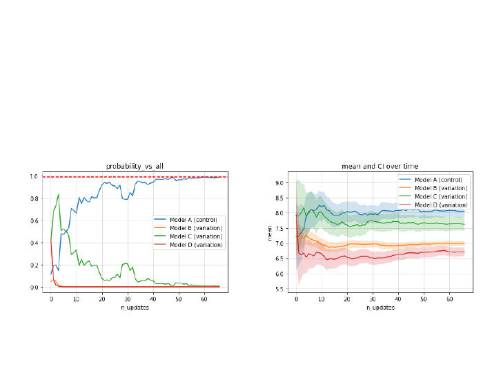
Bayesian experiment: normal distribution (4 / 4)
I
Reporting: visualize stopping rule metric over time (updates).
I
Reporting: visualize statistics over time (updates).
>>> experiment.plot_metric() >>> experiment.plot_stats()

32/33
Bibliography
M. Chen and Q. Shao.
Monte Carlo Estimation of Bayesian Credible and HPD Intervals.
Journal of Computational and Graphical Statistics, 8(1):69–92, 1999.
J. K. Kruschke.
Doing Bayesian Data Analysis: A Tutorial with R, JAGS and Stan.
Academic Press, Inc., Orlando, FL, USA, 2nd edition, 2015.
G. Navas-Palencia.
CPrior: Technical notes, 2019.
http://gnpalencia.org/cprior/formulas_models.html.
C. Stucchio.
Bayesian A/B Testing at VWO.
Visual Web Optimizer, 2015.

